Week 1: Foundations of Statistical Learning

Stat 577 — Statistical Learning Theory

Soumojit Das

Spring 2026

The Learning Problem

What Is Statistical Learning?

The core question: Given data, can we learn patterns that generalize to new observations?

Consider the relationship between inputs \(X\) and outputs \(Y\):

\[Y = f(X) + \varepsilon\]

where:

\(f\) is some fixed but unknown function
\(\varepsilon\) is a random error term with \(E[\varepsilon] = 0\)

Statistical learning is the set of approaches for estimating \(f\).

The Theory Behind the Magic

Before diving into formalism, consider what these methods have accomplished:

Cancer Diagnosis

20,000 gene expression features
Only 30–200 patient samples
Classify tumor types with >95% accuracy

Face Recognition

MIT’s breakthrough (1990s)
Thousands of pixel intensities
Real-time identification

Handwritten Digits

USPS mail sorting
256 grayscale features (16×16 image)
Human-level performance

Stock Prediction

Hundreds of economic indicators
Predict next-period returns
(With appropriate humility!)

The Common Thread

Each problem has the same structure: learn a function \(f\) from examples. But what is the theory behind such learning algorithms?

A Philosophical Aside

The framework \(Y = f(X) + \varepsilon\) is powerful but not innocent.

Hidden assumptions:

Additive noise: Real phenomena often have multiplicative or heteroskedastic errors
\(f\) exists: We’re defining \(f(x) = E[Y|X=x]\) — this is a modeling choice, not a discovery
\(\varepsilon\) is “error”: Implies there’s a “true” signal to recover — but what if nature is irreducibly stochastic?

The Right Attitude

Treat \(Y = f(X) + \varepsilon\) as a useful fiction — a framework for organizing our thinking, not a claim about reality.

The Ill-Posed Nature of Learning

Given training data, infinitely many functions pass through the same points.

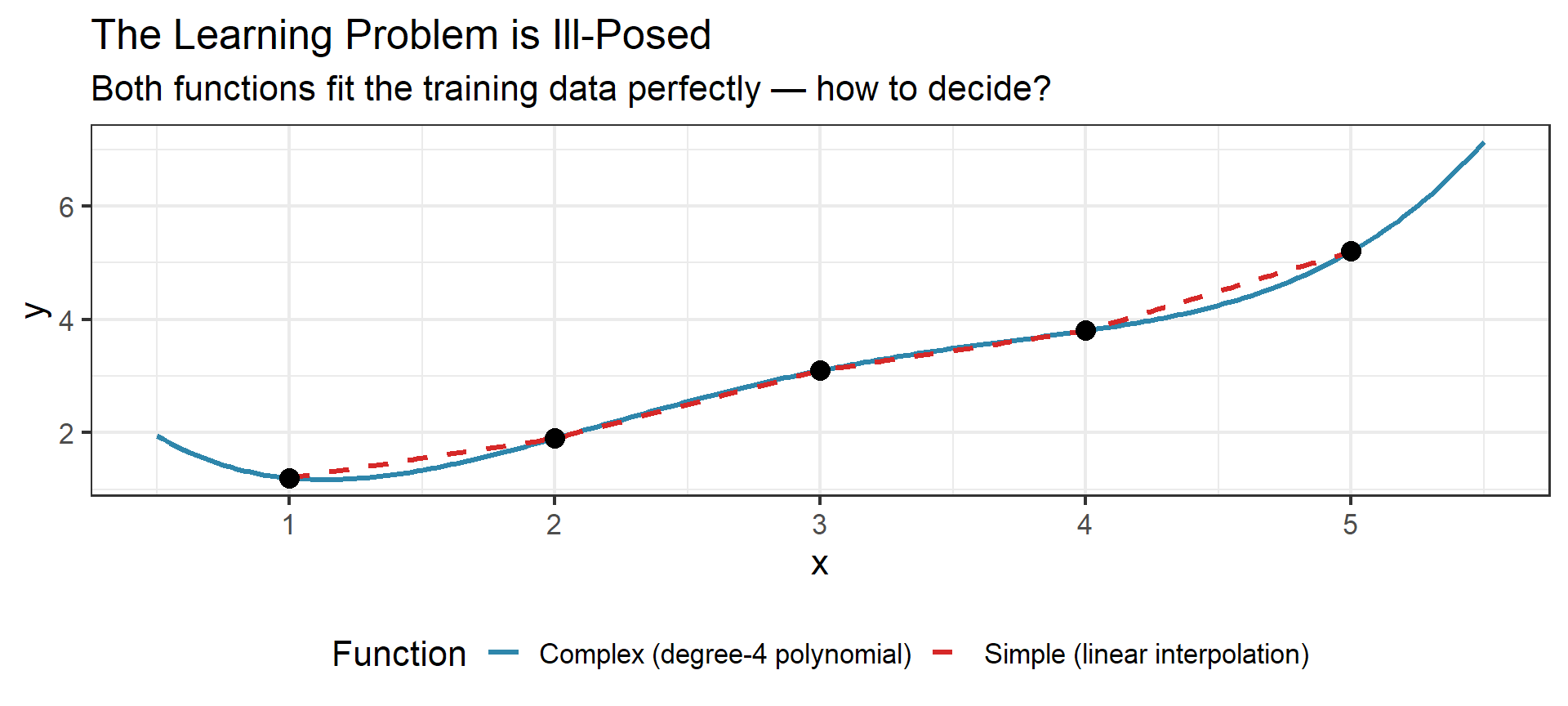
Occam’s Razor

Among all functions that fit the training data, prefer the simplest one.

This isn’t just aesthetic preference — it’s a statistical principle. Complex functions that fit training data perfectly often fail on new data. A good learning algorithm chooses the simplest \(f\) consistent with the evidence.

Why Estimate \(f\)?

Two main goals with different implications:

Prediction: We want \(\hat{Y} = \hat{f}(X)\) to be close to \(Y\)

Don’t care about the form of \(\hat{f}\)
Black box is fine if it predicts well
Example: predicting stock prices, disease risk

Inference: We want to understand how \(X\) affects \(Y\)

Which predictors are associated with the response?
What is the relationship (positive/negative, linear/nonlinear)?
Example: understanding drug effects, policy impacts

The Conflict

These goals can conflict. The best predictive model might be an uninterpretable neural network. The most interpretable model might predict poorly. This tension runs through the entire field.

Supervised vs Unsupervised Learning

Supervised Learning

Have both \(X\) and \(Y\) for training
Learn \(f: X \to Y\)
Regression: \(Y\) is continuous
Classification: \(Y\) is categorical

Examples: spam detection, house price prediction

Unsupervised Learning

Have only \(X\), no response \(Y\)
Find structure in the data
Clustering: group similar observations
Dimension reduction: find low-dimensional representation

Examples: customer segmentation, gene expression analysis

Scope

Most of this course focuses on supervised learning. But the boundary is blurry — semi-supervised methods use both labeled and unlabeled data.

No Free Lunch

A Fundamental Principle

“There is no free lunch in statistics: no one method dominates all others over all possible data sets.”

— ISLR, Chapter 2

What this means:

The “best” method depends on the specific problem
Linear regression beats neural nets on some datasets; neural nets win on others
Our job: understand when and why different methods work

This is why we study many methods, not just one. The course is about building a toolkit and knowing which tool to reach for.

Feature Vectors: The Language of Learning Machines

Any object — a patient, an image, a stock — can be summarized as a string of numbers.

The key insight: Once we represent objects as vectors \(\mathbf{x} \in \mathbb{R}^p\), they become points in high-dimensional space.

Classification becomes: finding a surface that separates points
Regression becomes: finding a surface that passes through points
Clustering becomes: identifying clumps of nearby points

Geometrization of Data

Statistical learning is fundamentally geometric. Every method we study is a different way of carving up or smoothing over feature space.

Notation Setup

Our Notation Convention (ISLR/ESL style)

Symbol	Meaning
\(n\)	Sample size (number of observations)
\(p\)	Number of predictors/features
\(\mathbf{X} \in \mathbb{R}^{n \times p}\)	Design matrix
\(\mathbf{y} \in \mathbb{R}^n\)	Response vector
\(\mathbf{x}_i \in \mathbb{R}^p\)	Feature vector for observation \(i\) (row of \(\mathbf{X}\))
\((x_i, y_i)\)	\(i\)th observation pair
\(\hat{f}\)	Estimated function
\(\hat{y}\)	Predicted value

Loss Functions & Optimal Predictors

Measuring Prediction Error

To evaluate how well \(\hat{f}\) approximates \(f\), we need a loss function \(L(y, \hat{y})\).

Common loss functions:

Name	Formula	Optimal Predictor
Squared loss (\(L_2\))	\((y - \hat{y})^2\)	Conditional mean
Absolute loss (\(L_1\))	\(\|y - \hat{y}\|\)	Conditional median
0-1 loss	\(\mathbf{1}(y \neq \hat{y})\)	Bayes classifier

The choice of loss function determines what “optimal” means.

Expected Prediction Error

Definition: Expected Prediction Error (EPE)

For a loss function \(L\) and predictor \(\hat{f}\):

\[\text{EPE}(\hat{f}) = E_{X,Y}[L(Y, \hat{f}(X))]\]

This averages over both the distribution of \(X\) and the conditional distribution of \(Y|X\).

For squared loss, we can decompose EPE pointwise:

\[\text{EPE}(\hat{f}) = E_X\left[ E_{Y|X}[(Y - \hat{f}(X))^2 | X] \right]\]

Optimal Predictor Under Squared Loss

Theorem: The function minimizing EPE under squared loss is the conditional expectation:

\[f^*(x) = E[Y | X = x]\]

Proof sketch: \[E[(Y - c)^2 | X = x] = E[Y^2|X=x] - 2cE[Y|X=x] + c^2\]

Take derivative w.r.t. \(c\), set to zero: \[-2E[Y|X=x] + 2c = 0 \implies c = E[Y|X=x]\]

Intuition

The conditional mean is the “center of mass” of \(Y\) given \(X=x\) — it minimizes the average squared distance.

Optimal Predictor Under Absolute Loss

Theorem: The function minimizing EPE under absolute loss is the conditional median:

\[f^*(x) = \text{median}(Y | X = x)\]

Why Median?

The median minimizes the sum of absolute deviations
More robust to outliers than the mean
Useful when extreme values shouldn’t dominate

Why Use \(L_1\)? Robustness to Outliers

The Lesson

One outlier shifts the mean by 2 but the median by only 0.1.

When outliers are expected (income data, sensor errors, etc.), \(L_1\) loss gives more robust predictions.

The Bayes Classifier (Classification)

For classification with 0-1 loss, the optimal classifier assigns each \(x\) to the most probable class:

\[f^*(x) = \arg\max_{g} P(Y = g | X = x)\]

Bayes Error Rate

The error rate of the Bayes classifier is:

\[R^* = 1 - E_X[\max_g P(Y = g | X)]\]

This is the irreducible error — no classifier can do better.

Hmm, why not use it then?

Problem:

We don’t know the true (population quantity of interest) \(P(Y = g | X)\) — must estimate it from data (sample).
Every classification method we study — logistic regression, LDA, k-NN, random forests, neural networks — is just a different way of estimating these posterior probabilities.
The Bayes Classifier is what we’d use if we had perfect knowledge of the data-generating process.

Visualizing the Bayes Classifier

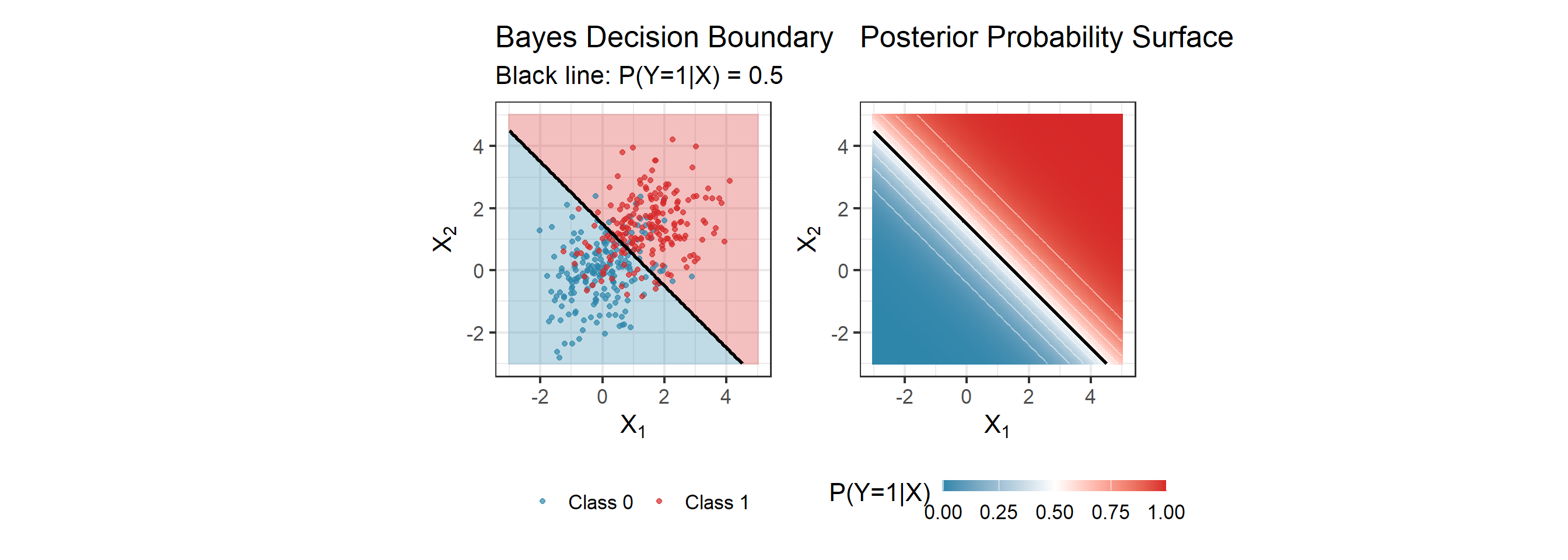
Reading This Plot

Left: Points near the boundary are hard to classify — even the optimal classifier makes mistakes there
Right: The gradient shows uncertainty. Near the boundary, \(P(Y=1|X) \approx 0.5\) — maximum uncertainty
Bayes error: The shaded overlap region where even perfect knowledge of \(P(Y|X)\) leads to errors

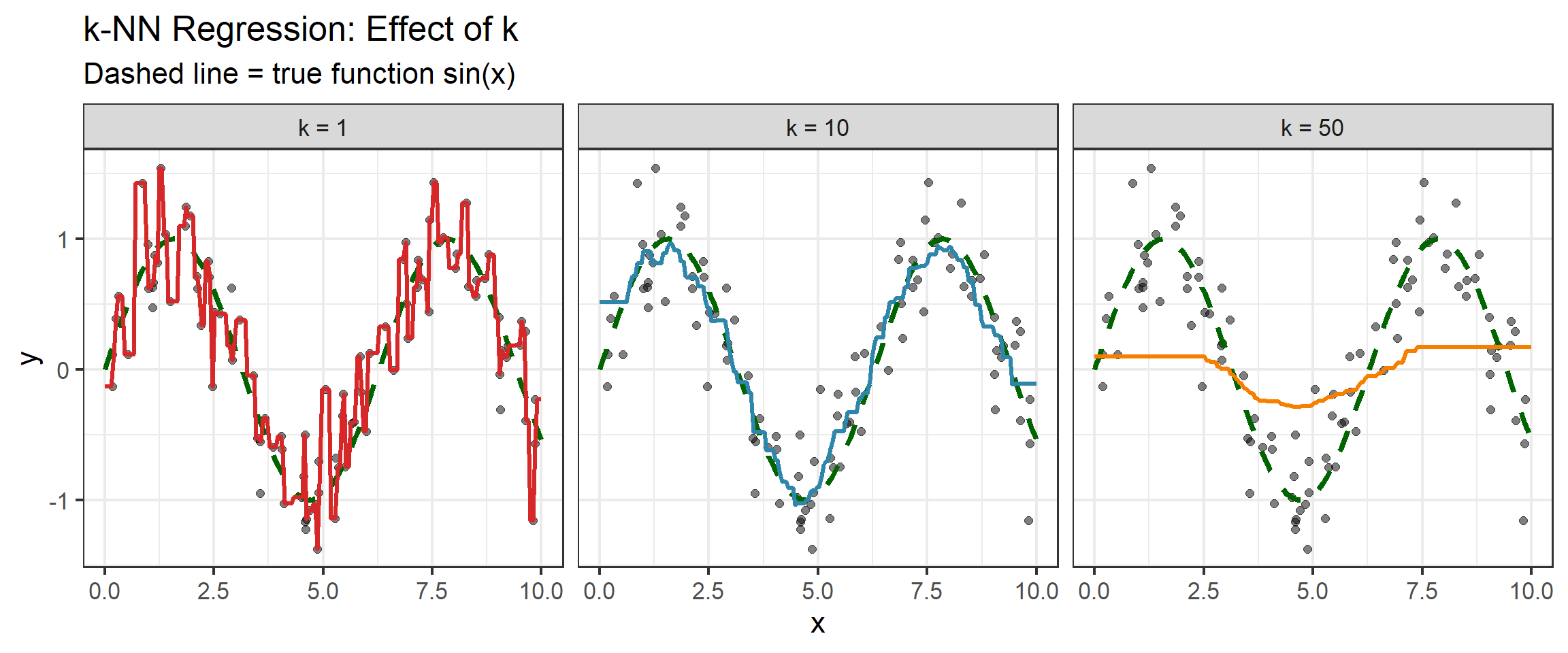
Example: k-Nearest Neighbors

A simple, intuitive approach to estimate \(f(x)\):

Find the \(k\) training points closest to \(x\)
For regression: average their \(y\) values
For classification: majority vote

\[\hat{f}(x) = \frac{1}{k} \sum_{x_i \in N_k(x)} y_i\]

where \(N_k(x)\) is the set of \(k\) nearest neighbors of \(x\).

Key Question

How should we choose \(k\)? This is a model complexity parameter.

k-NN: Effect of \(k\)

k-NN: Practical Considerations

Boundary Effects

At the edges of the data (\(x \approx 0\) or \(x \approx 10\)), k-NN effectively uses a “half-neighborhood” — all \(k\) neighbors come from one direction. This causes:

Increased bias at boundaries
Predictions pulled toward the interior

Other practical issues:

Computational cost: Finding neighbors requires \(O(n)\) comparisons per prediction (or \(O(\log n)\) with KD-trees)
Feature scaling: Distances depend on units — always standardize!
Choosing \(k\): Use cross-validation (we’ll formalize this soon)

Two Philosophies: Global vs Local

Linear Regression

“Globally linear”

Assumes \(f(x) \approx \beta_0 + \boldsymbol{\beta}^T\mathbf{x}\) everywhere
One model fits all regions of the input space
Very strong assumption — but stable estimates
Few parameters to estimate

k-Nearest Neighbors

“Locally constant”

Assumes \(f(x) \approx\) constant in small neighborhoods
Adapts to local structure
Very weak assumption — but noisy estimates
Effectively uses all data as “parameters”

The Tradeoff Emerges

Strong assumptions (linear) → Lower variance, potentially higher bias

Weak assumptions (k-NN) → Lower bias, higher variance

This tension is the heart of statistical learning.

Where This Course Lives

The methods we study occupy the middle ground between these extremes:

Method	Structure	Locality	This Course
Linear regression	Global, rigid	None	Week 2
Ridge/Lasso	Global, regularized	None	Week 3
Splines, GAMs	Semi-local, smooth	Moderate	Week 5
Trees, forests	Adaptive partitions	Local	Week 6
SVM	Global (kernel-dependent)	Varies	Week 7
Neural networks	Hierarchical	Learned	Weeks 8–12
k-NN	Local, unstructured	High	Week 1 (today)

The Course Arc

We’ll build from strong assumptions (linear models) toward flexible methods (neural networks), always asking: what assumptions does this method make, and when do they help or hurt?

Bias-Variance Decomposition

The Fundamental Tradeoff

We’ve seen that linear models make strong assumptions (low variance, potential bias) while k-NN makes weak assumptions (low bias, high variance).

But can we make this precise? What exactly do “bias” and “variance” mean, and how do they affect prediction error?

Imagine we could repeatedly sample training sets and fit \(\hat{f}\).

For a fixed test point \(x_0\), the expected prediction error has three components:

\[E[(Y - \hat{f}(x_0))^2] = \underbrace{\sigma^2}_{\text{Irreducible}} + \underbrace{[\text{Bias}(\hat{f}(x_0))]^2}_{\text{Bias}^2} + \underbrace{\text{Var}(\hat{f}(x_0))}_{\text{Variance}}\]

Key Insight

We cannot minimize bias and variance simultaneously — this is the bias-variance tradeoff.

Derivation: Setting Up

Let \(Y = f(x_0) + \varepsilon\) where \(E[\varepsilon] = 0\) and \(\text{Var}(\varepsilon) = \sigma^2\).

The expected squared error at \(x_0\) (expectation over training data and \(\varepsilon\)):

\[\text{Err}(x_0) = E[(Y - \hat{f}(x_0))^2]\]

Write \(Y - \hat{f}(x_0) = (Y - f(x_0)) + (f(x_0) - \hat{f}(x_0))\)

\[= \varepsilon + (f(x_0) - \hat{f}(x_0))\]

Derivation: Expanding the Square

\[E[(Y - \hat{f}(x_0))^2] = E[(\varepsilon + f(x_0) - \hat{f}(x_0))^2]\]

Expand: \[= E[\varepsilon^2] + 2E[\varepsilon(f(x_0) - \hat{f}(x_0))] + E[(f(x_0) - \hat{f}(x_0))^2]\]

Since \(\varepsilon\) is independent of \(\hat{f}\) and has mean 0:

\[= \sigma^2 + 0 + E[(f(x_0) - \hat{f}(x_0))^2]\]

Derivation: Decomposing the Second Term

Now decompose \(E[(f(x_0) - \hat{f}(x_0))^2]\).

Add and subtract \(E[\hat{f}(x_0)]\):

\[= E[(f(x_0) - E[\hat{f}(x_0)] + E[\hat{f}(x_0)] - \hat{f}(x_0))^2]\]

Let \(a = f(x_0) - E[\hat{f}(x_0)]\) (a constant) and \(b = E[\hat{f}(x_0)] - \hat{f}(x_0)\) (random).

\[= E[(a + b)^2] = a^2 + 2aE[b] + E[b^2]\]

Derivation: Final Result

Note that \(E[b] = E[E[\hat{f}(x_0)] - \hat{f}(x_0)] = 0\).

So: \[E[(f(x_0) - \hat{f}(x_0))^2] = a^2 + E[b^2]\]

\[= (f(x_0) - E[\hat{f}(x_0)])^2 + E[(E[\hat{f}(x_0)] - \hat{f}(x_0))^2]\]

Bias-Variance Decomposition

\[E[(Y - \hat{f}(x_0))^2] = \sigma^2 + \underbrace{[f(x_0) - E[\hat{f}(x_0)]]^2}_{\text{Bias}^2(\hat{f}(x_0))} + \underbrace{\text{Var}(\hat{f}(x_0))}_{\text{Variance}}\]

What Each Term Means

Irreducible Error \(\sigma^2\)

Noise in the data itself
Cannot be reduced
Sets a floor for prediction error

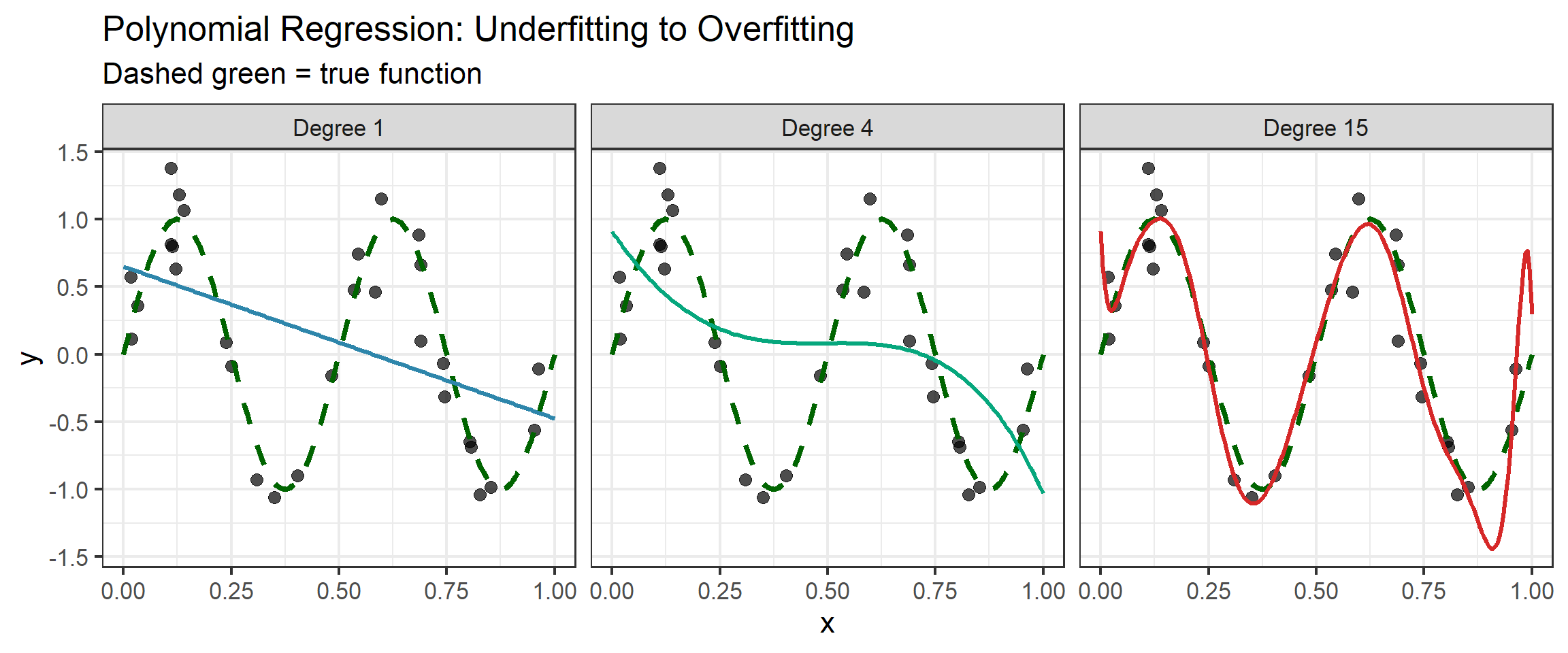
Bias\(^2\)

Error from wrong model assumptions
Simple models → high bias
“Underfitting”

Variance

Sensitivity to training data
Complex models → high variance
“Overfitting”

The Tradeoff

More flexible models: lower bias, higher variance
Less flexible models: higher bias, lower variance
Goal: find the sweet spot

But…

This U-shaped picture is a mental model, not a theorem. Double descent (Week 8) shows the story is richer. The bias-variance decomposition is a framework for thinking, not a universal law.

The Dartboard Analogy

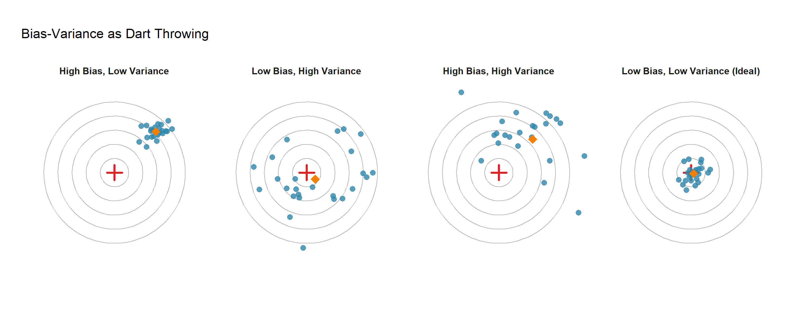
The Analogy

Bias = How far is your average throw from the bullseye? (Systematic error)
Variance = How spread out are your throws? (Consistency)
Goal = Low bias AND low variance (rightmost panel)

The U-Shaped Test Error Curve

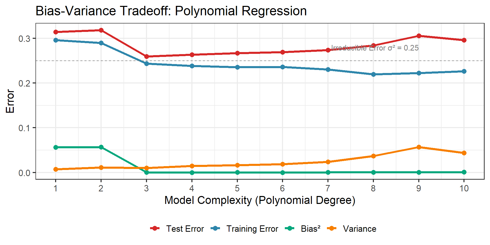
Training Error vs Test Error

Training Error

Computed on data used to fit model
Always decreases with complexity
Optimistic estimate of true error
Can reach zero with enough flexibility

Test Error

Computed on new, unseen data
U-shaped curve
Minimum at optimal complexity
This is what we actually care about!

Key Lesson

Never use training error to select model complexity!

Polynomial Fitting Demo

Curse of Dimensionality

The High-Dimensional Challenge

As dimension \(p\) increases, our intuition about space breaks down.

The problem: Local methods (like k-NN) assume we can find “nearby” points.

In high dimensions:

Data becomes sparse
“Nearby” points aren’t so near
Local neighborhoods become global

This Isn’t Hypothetical

Consider real applications we mentioned earlier:

Application	Dimension \(p\)	Typical Sample Size \(n\)
Gene expression (cancer)	5,000 – 20,000	30 – 200
Face recognition	10,000+ (pixels)	100 – 1,000
Text classification	50,000+ (vocabulary)	1,000 – 10,000
Financial indicators	100 – 1,000	250 (trading days/year)

The Uncomfortable Reality

In most modern applications, \(p \gg n\) — we have far more features than observations.

Classical statistics (designed for \(n \gg p\)) doesn’t directly apply. This is where statistical learning theory becomes essential.

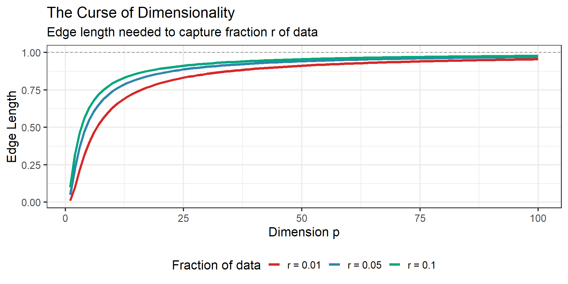
Edge Length to Capture \(r\) Fraction of Data

Consider data uniformly distributed in a \(p\)-dimensional unit hypercube.

To capture a fraction \(r\) of the data in a hypercubic neighborhood centered at a point, we need edge length:

\[e_p(r) = r^{1/p}\]

Dimension \(p\)	Edge length for \(r = 0.01\)	Edge length for \(r = 0.1\)
1	0.01	0.10
2	0.10	0.32
10	0.63	0.79
100	0.955	0.977

The Curse

In high dimensions, even small neighborhoods span most of the data range!

Visualizing the Curse

Why Local Methods Struggle

In low dimensions:

k nearest neighbors are genuinely local
Can estimate \(f(x)\) by averaging nearby points
Works well for smooth functions

In high dimensions:

“Nearest” neighbors may be far away
Neighborhoods become nearly as large as the whole space
Effectively averaging over dissimilar points

Sample size requirement: To maintain constant density of points, need \(n = O(c^p)\) samples!

How Bad Is It? A Calculation

Suppose we want training points dense enough that the nearest neighbor is within 1% of each axis (linear density = 100).

Required sample size:

Dimension \(p\)	Required \(n = 100^p\)
1	100
2	10,000
5	10 billion
10	\(10^{20}\) (more than atoms in a gram of matter)

The Fundamental Lesson

In high dimensions, there is no substitute for assumptions.

We cannot simply “collect more data” — the required sample size grows exponentially. Instead, we must impose structure: linearity, sparsity, smoothness, or low intrinsic dimension.

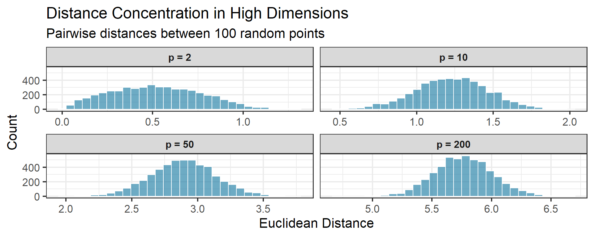
Distance Concentration

An even stranger phenomenon: in high dimensions, all pairwise distances become nearly equal.

For \(n\) points uniformly distributed in the unit hypercube:

\[\frac{d_{\max} - d_{\min}}{d_{\min}} \to 0 \quad \text{as } p \to \infty\]

Implication

If all points are equidistant, the concept of “nearest neighbor” becomes meaningless!

Volume of a Hypersphere

Another perspective: the volume of a unit ball shrinks rapidly.

Volume of unit ball in \(p\) dimensions:

\[V_p(1) = \frac{\pi^{p/2}}{\Gamma(p/2 + 1)}\]

Dimension \(p\)	Volume
2	\(\pi \approx 3.14\)
3	\(\frac{4\pi}{3} \approx 4.19\)
10	\(\approx 2.55\)
20	\(\approx 0.026\)
100	\(\approx 10^{-40}\)

Most of the “volume” is in the corners of the hypercube!

Concentration of Measure

Perhaps the most counterintuitive result: most of a high-dimensional sphere’s volume is near its surface.

For a unit ball in \(p\) dimensions, the fraction of volume within distance \(\epsilon\) of the surface is:

\[\text{Fraction in shell} = 1 - (1 - \epsilon)^p \approx 1 - e^{-p\epsilon} \text{ for large } p\]

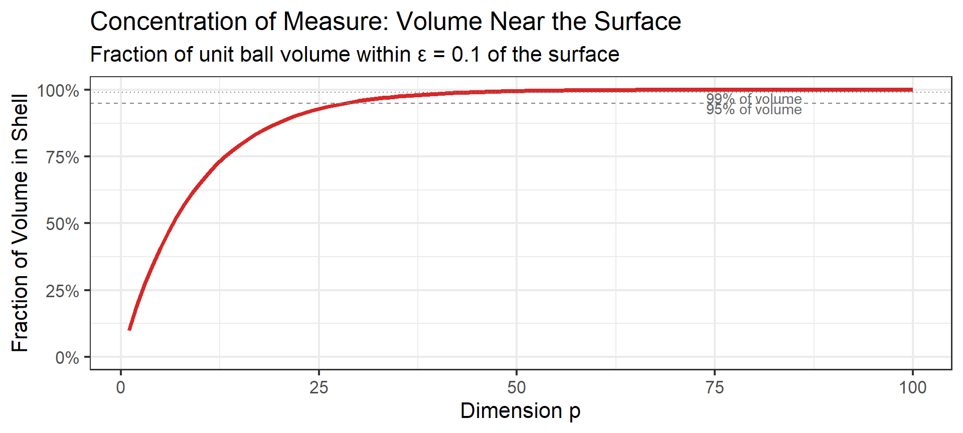
What This Means

In high dimensions:

Almost all random points lie near the “edge” of any bounded region
The “interior” is essentially empty
Uniformly distributed points don’t fill space — they concentrate on the boundary

This is why sampling in high dimensions feels fundamentally different.

What Can We Do?

The curse of dimensionality tells us we need assumptions to learn in high dimensions.

Common structural assumptions:

Smoothness: \(f\) doesn’t change too rapidly
Sparsity: Only a few predictors matter
Low intrinsic dimension: Data lies on a lower-dimensional manifold
Linearity: \(f\) is approximately linear

Key Insight

Statistical learning is about choosing the right structural assumptions for your problem.

Preview: Modern Phenomena

Beyond the Classical View

The bias-variance tradeoff suggests: don’t overfit!

Classical advice:

Use fewer parameters than data points
Regularize heavily
Stop before fitting noise

But modern deep learning:

Uses millions of parameters
Often fits training data perfectly
Still generalizes well!

What’s going on?

Double Descent

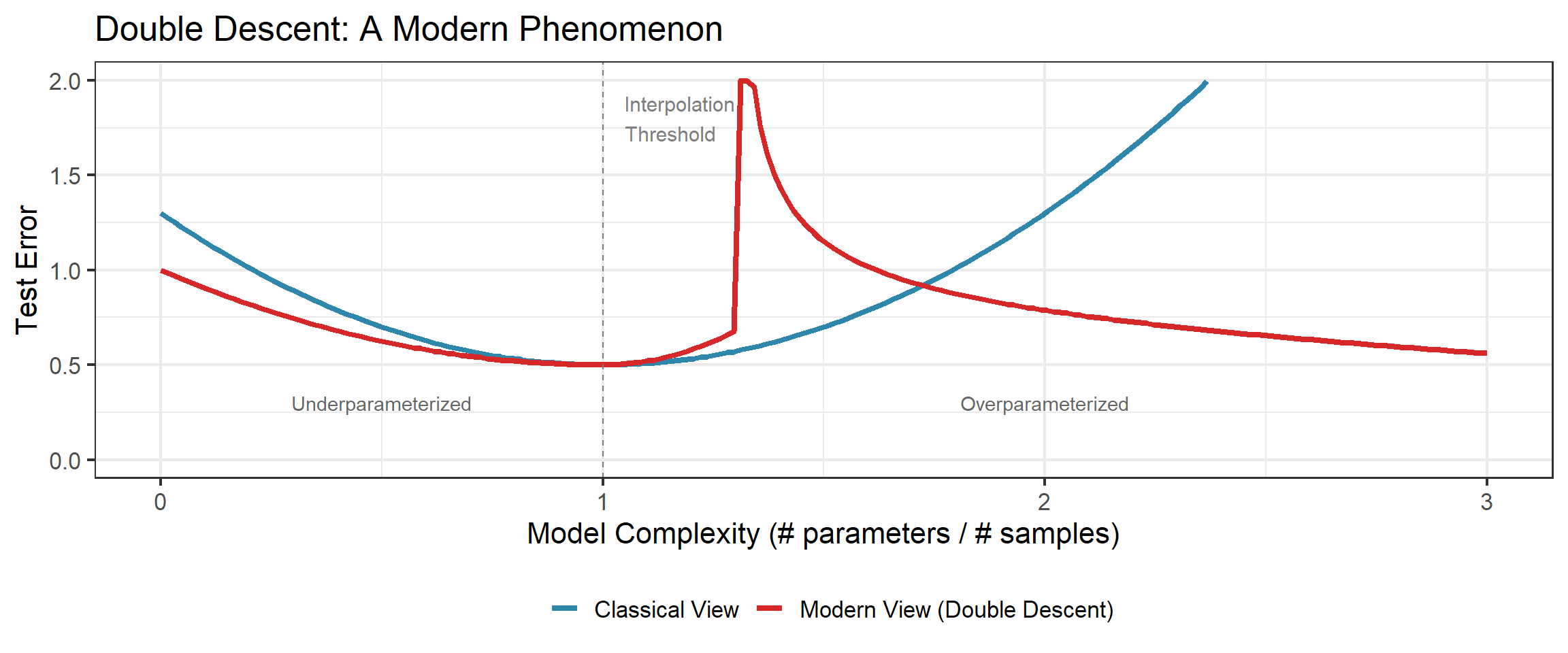
What Is Double Descent?

The Phenomenon

Test error can decrease again after the interpolation threshold — when models have enough capacity to perfectly fit training data.

Three regimes:

Underparameterized: Classical bias-variance tradeoff applies
Interpolation threshold: Peak error (barely enough capacity)
Overparameterized: Error decreases again!

We’ll revisit this in Week 8 (Neural Networks).

Why Does Overparameterization Help?

Several (still debated!) explanations:

Implicit regularization: Gradient descent finds “simple” solutions even in overparameterized models
Multiple interpolating solutions: With many parameters, some that fit training data also generalize
Smoothness: Overparameterized models can be smoother than barely-fitting ones

Open Question

We don’t fully understand this yet! Active area of research.

Summary

Key Takeaways

Feature vectors are the language of learning machines — any object becomes a point in high-dimensional space
The learning problem is ill-posed — many functions fit the data; Occam’s razor says prefer the simplest
Loss functions define what “optimal” means:
- Squared loss → conditional mean
- Absolute loss → conditional median (robust to outliers)
- 0-1 loss → Bayes classifier
Bias-variance decomposition: \[\text{EPE} = \sigma^2 + \text{Bias}^2 + \text{Variance}\]
Curse of dimensionality: In high dimensions (\(p \gg n\)), local methods fail — we need structural assumptions
Modern twist: Double descent shows the story is richer than the classical U-curve — stay curious!

Looking Ahead

Next week: Linear Models & Least Squares

The workhorse of statistical learning
Matrix formulation and geometry
Hat matrix and projection interpretation
Gauss-Markov theorem (proof sketch)
Distributional properties

Preparation:

Read: ISLR Chapter 3
Optional: ESL 3.1-3.2