set.seed(577)
n <- 200; p <- 50
X <- matrix(rnorm(n * p), n, p)
beta_true <- c(rep(2, 5), rep(0, 45))
y <- X %*% beta_true + rnorm(n, sd = 2)
dat <- data.frame(y = y, X)
# Manual 10-fold CV: compare models using first d predictors (d = 1,...,15)
k <- 10
folds <- sample(rep(1:k, length.out = n))
n_vars <- 1:15
cv_errors <- matrix(NA, k, length(n_vars))
for (d in seq_along(n_vars)) {
pred_names <- paste0("X", 1:n_vars[d])
fmla <- as.formula(paste("y ~", paste(pred_names, collapse = " + ")))
for (j in 1:k) {
train_idx <- which(folds != j)
test_idx <- which(folds == j)
fit <- lm(fmla, data = dat[train_idx, ])
pred <- predict(fit, newdata = dat[test_idx, ])
cv_errors[j, d] <- mean((dat$y[test_idx] - pred)^2)
}
}
cv_mean <- colMeans(cv_errors)
cv_se <- apply(cv_errors, 2, sd) / sqrt(k)
cv_results <- tibble(
n_predictors = n_vars,
cv_mean = cv_mean,
cv_lo = cv_mean - cv_se,
cv_hi = cv_mean + cv_se
)
p_kfold <- ggplot(cv_results, aes(x = n_predictors, y = cv_mean)) +
geom_ribbon(aes(ymin = cv_lo, ymax = cv_hi), alpha = 0.2, fill = colors["blue"]) +
geom_line(linewidth = 1.2, color = colors["blue"]) +
geom_point(size = 3, color = colors["blue"]) +
geom_vline(xintercept = n_vars[which.min(cv_mean)], linetype = "dashed", color = colors["red"]) +
annotate("text", x = n_vars[which.min(cv_mean)] + 0.3, y = max(cv_mean) * 0.97,
label = paste0("Optimal: ", n_vars[which.min(cv_mean)], " predictors"),
color = colors["red"], hjust = 0, size = 4.5) +
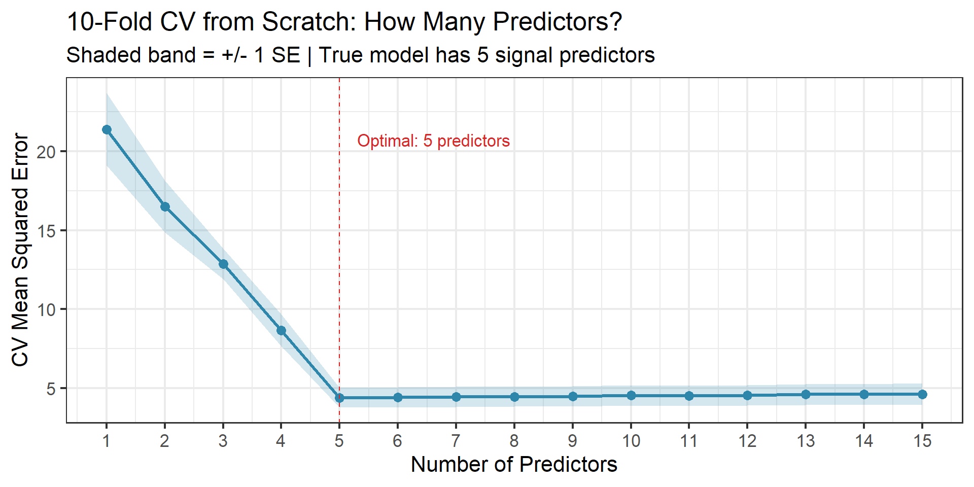
labs(title = "10-Fold CV from Scratch: How Many Predictors?",
subtitle = "Shaded band = +/- 1 SE | True model has 5 signal predictors",
x = "Number of Predictors", y = "CV Mean Squared Error") +
scale_x_continuous(breaks = n_vars) +
theme_bw(base_size = 16)
ggsave(file.path(fig_dir, "07_kfold_scratch.png"), p_kfold, width = 10, height = 5, dpi = 150)
p_kfoldWeeks 4–5: Resampling, Model Selection & Conformal Prediction
Stat 577 — Statistical Learning Theory
Spring 2026
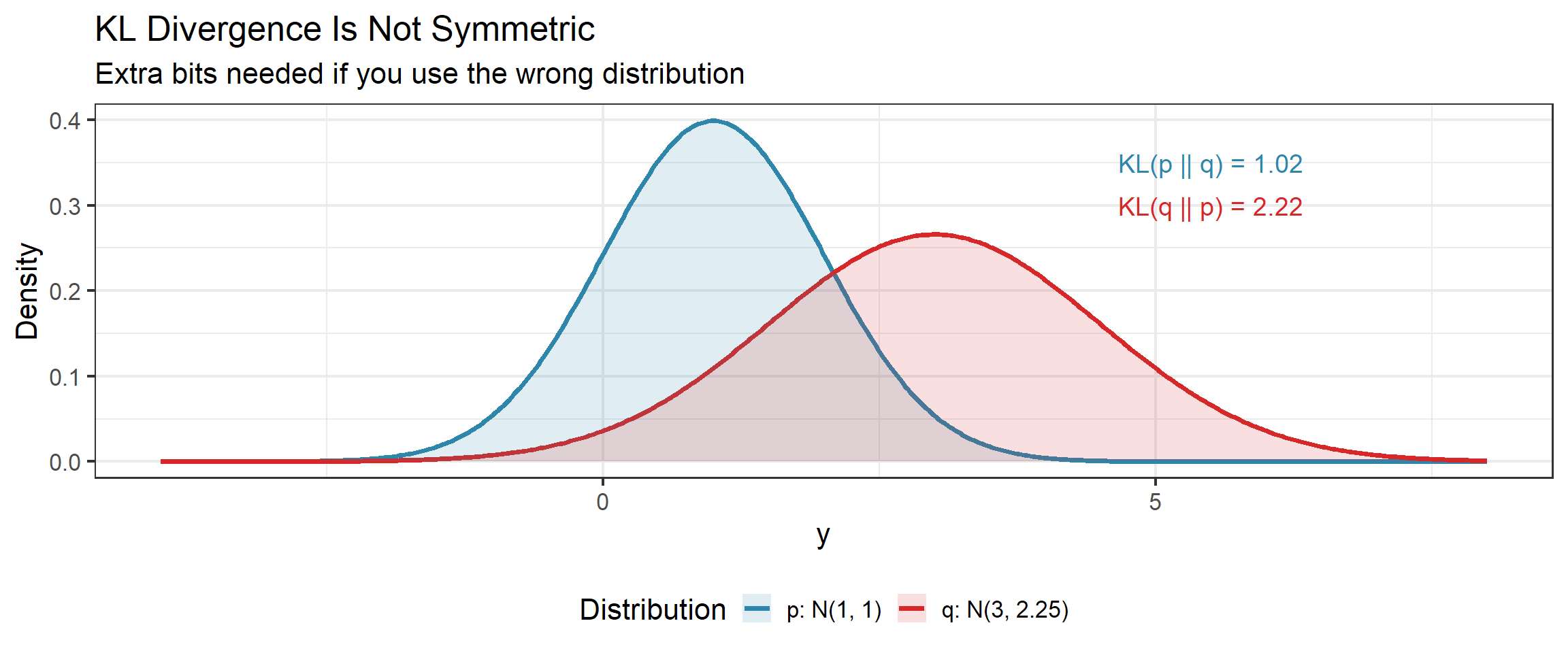
KL Divergence: Visual Intuition
Effective df for Ridge: Visualization
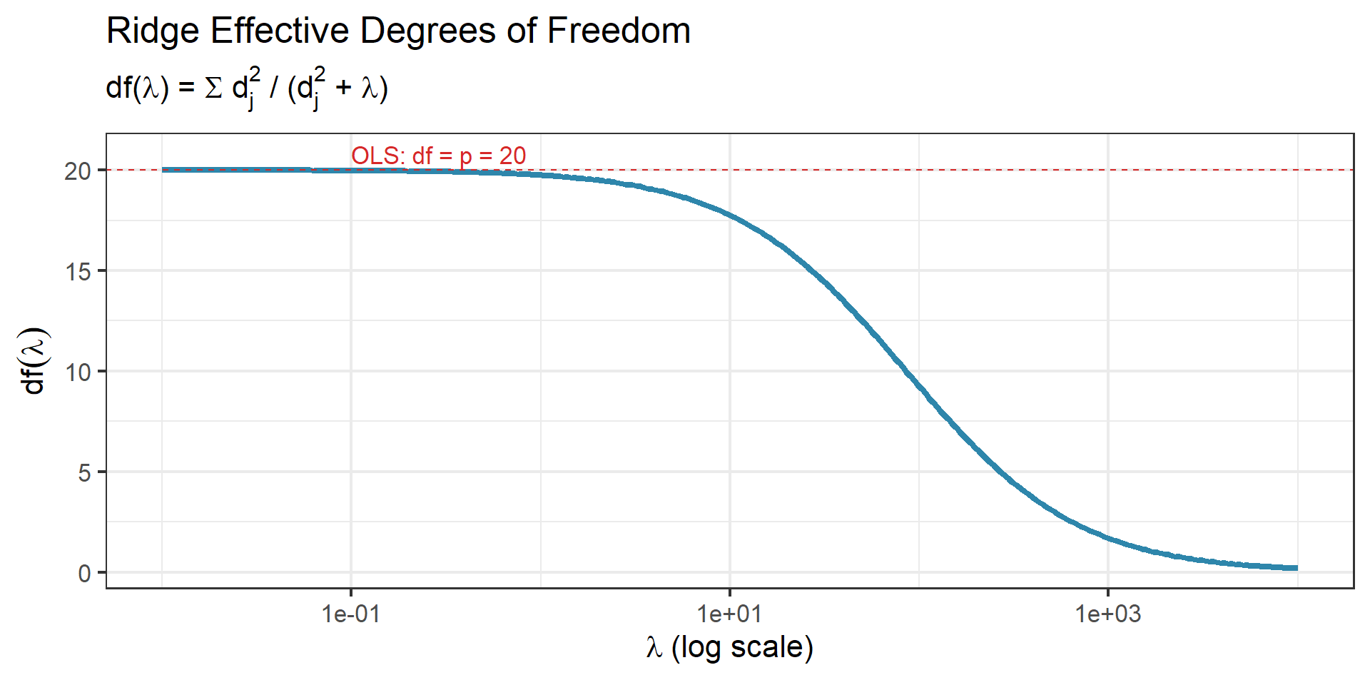
Recall from Week 3
We saw effective df in the context of shrinkage along principal components. Each singular direction contributes \(d_j^2/(d_j^2 + \lambda) \in [0, 1]\) degrees of freedom — a fractional count of how much that direction is being used.
Code Demo: k-Fold CV from Scratch
Code Demo: k-Fold CV with glmnet
set.seed(577)
n <- 200; p <- 50
X <- matrix(rnorm(n * p), n, p)
beta_true <- c(rep(2, 5), rep(0, 45))
y <- X %*% beta_true + rnorm(n, sd = 2)

# 10-fold CV for Lasso
cv_fit <- cv.glmnet(X, y, alpha = 1, nfolds = 10)

# Rebuild CV curve in ggplot2 for consistent styling
cv_df <- tibble(
  lambda = cv_fit$lambda,
  cvm    = cv_fit$cvm,
  cvup   = cv_fit$cvup,
  cvlo   = cv_fit$cvlo,
  nzero  = cv_fit$nzero
)

p_cv <- ggplot(cv_df, aes(x = log(lambda), y = cvm)) +
  geom_ribbon(aes(ymin = cvlo, ymax = cvup), alpha = 0.15, fill = colors["blue"]) +
  geom_point(color = colors["red"], size = 1.8) +
  geom_vline(xintercept = log(cv_fit$lambda.min), linetype = "dashed", color = colors["blue"]) +
  geom_vline(xintercept = log(cv_fit$lambda.1se), linetype = "dashed", color = colors["orange"]) +
  annotate("text", x = log(cv_fit$lambda.min), y = max(cv_df$cvup) * 0.95,
           label = "lambda[min]", parse = TRUE, hjust = 1.1, color = colors["blue"], size = 4.5) +
  annotate("text", x = log(cv_fit$lambda.1se), y = max(cv_df$cvup) * 0.95,
           label = "lambda['1se']", parse = TRUE, hjust = -0.1, color = colors["orange"], size = 4.5) +
  labs(title = "10-Fold Cross-Validation for Lasso",
       subtitle = "Error bars = +/- 1 SE | Dashed lines = lambda_min and lambda_1se",
       x = expression(log(lambda)), y = "Mean Squared Error (CV)") +
  theme_bw(base_size = 16) +
  theme(plot.title = element_text(size = 14))

ggsave(file.path(fig_dir, "05_cv_glmnet.png"), p_cv, width = 10, height = 5, dpi = 150)
p_cv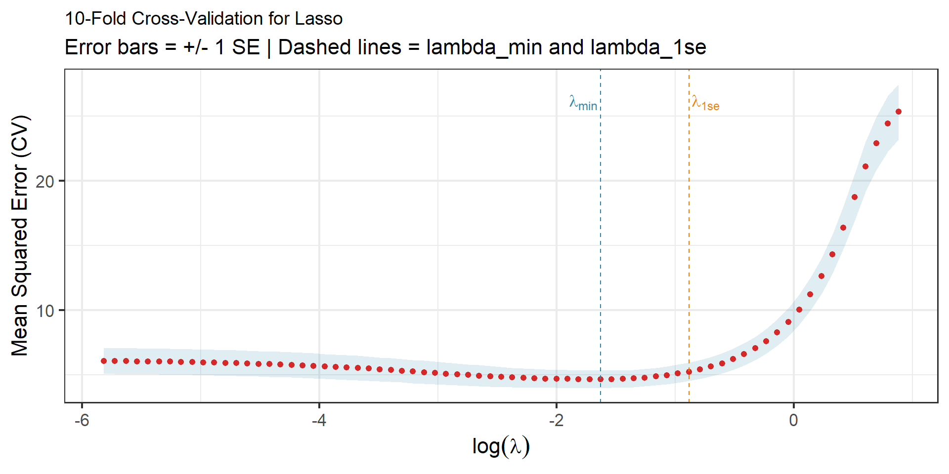
Reading the Plot
- Left dashed line: \(\lambda_{\min}\) — minimizes CV error
- Right dashed line: \(\lambda_{\text{1se}}\) — most regularized model within 1 SE of the minimum
- The x-axis is \(\log(\lambda)\), so regularization increases from left to right
Bootstrap Demo: Ridge Coefficient Uncertainty
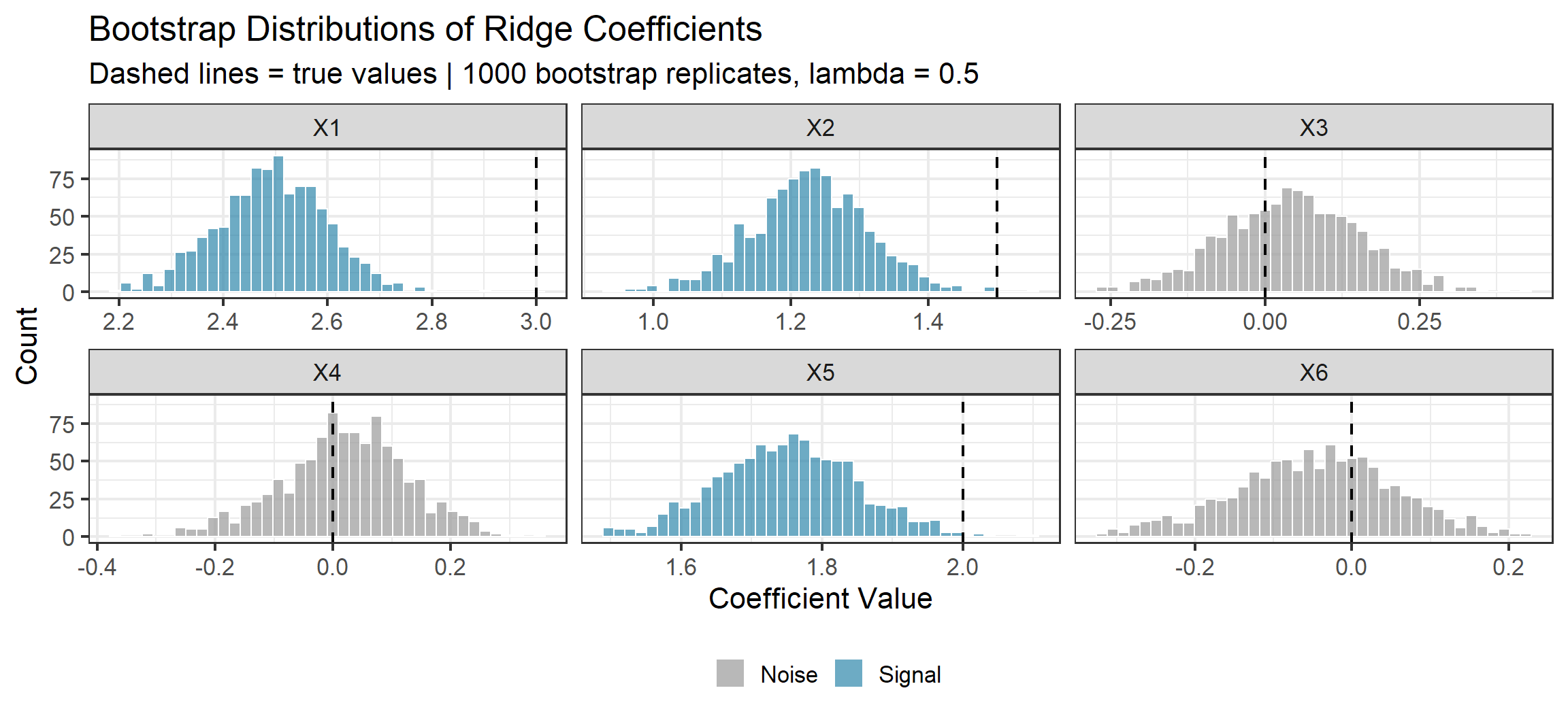
Notice the Shrinkage
The bootstrap distributions for the signal coefficients (\(X_1, X_2, X_5\)) are centered below their true values. This is Ridge doing its job — biasing toward zero in exchange for lower variance.
Bootstrap CI Demo: Median Regression Coefficient
set.seed(577)
n <- 100; p <- 10
X <- matrix(rnorm(n * p), n, p)
beta_true <- c(3, 1.5, 0, 0, 2, rep(0, 5))
y <- X %*% beta_true + rnorm(n)

# Point estimate: Ridge coefficient for X1
fit_full <- glmnet(X, y, alpha = 0, lambda = 0.5)
theta_hat <- as.vector(coef(fit_full))[-1][1]  # X1 coefficient

# Bootstrap
B <- 2000
boot_theta <- numeric(B)
for (b in 1:B) {
  idx <- sample(1:n, n, replace = TRUE)
  fit_b <- glmnet(X[idx, ], y[idx], alpha = 0, lambda = 0.5)
  boot_theta[b] <- as.vector(coef(fit_b))[-1][1]
}

# Three types of 95% CIs
alpha <- 0.05
q_lo <- quantile(boot_theta, alpha / 2)
q_hi <- quantile(boot_theta, 1 - alpha / 2)

ci_percentile <- c(q_lo, q_hi)
ci_basic <- c(2 * theta_hat - q_hi, 2 * theta_hat - q_lo)

ci_df <- tibble(
  Method = c("Percentile", "Basic (Pivotal)"),
  lo = c(ci_percentile[1], ci_basic[1]),
  hi = c(ci_percentile[2], ci_basic[2]),
  ypos = c(-0.15, 0)
)

p_ci <- ggplot() +
  geom_histogram(aes(x = boot_theta, y = after_stat(density)),
                 bins = 50, fill = colors["blue"], alpha = 0.5, color = "white") +
  geom_vline(xintercept = theta_hat, linewidth = 1, color = "black") +
  geom_vline(xintercept = 3, linewidth = 1, linetype = "dashed", color = colors["red"]) +
  geom_segment(data = ci_df, aes(x = lo, xend = hi, y = ypos, yend = ypos, color = Method),
               linewidth = 2) +
  geom_point(data = ci_df, aes(x = lo, y = ypos, color = Method), size = 3) +
  geom_point(data = ci_df, aes(x = hi, y = ypos, color = Method), size = 3) +
  scale_color_manual(values = c("Percentile" = colors["green"], "Basic (Pivotal)" = colors["orange"])) +
  annotate("text", x = 3.05, y = 2.5, label = "'True' ~ beta[1] == 3",
           parse = TRUE, color = colors["red"], hjust = 0, size = 4.5) +
  annotate("text", x = theta_hat + 0.05, y = 2.8,
           label = paste0("hat(theta) == ", round(theta_hat, 2)),
           parse = TRUE, hjust = 0, size = 4.5) +
  labs(title = "Bootstrap Confidence Intervals for Ridge Coefficient (X1)",
       subtitle = "2000 bootstrap replicates | lambda = 0.5 | 95% confidence level",
       x = "Coefficient Value", y = "Density") +
  theme_bw(base_size = 16) +
  theme(legend.position = "bottom")

ggsave(file.path(fig_dir, "06_bootstrap_ci.png"), p_ci, width = 10, height = 5, dpi = 150)
p_ci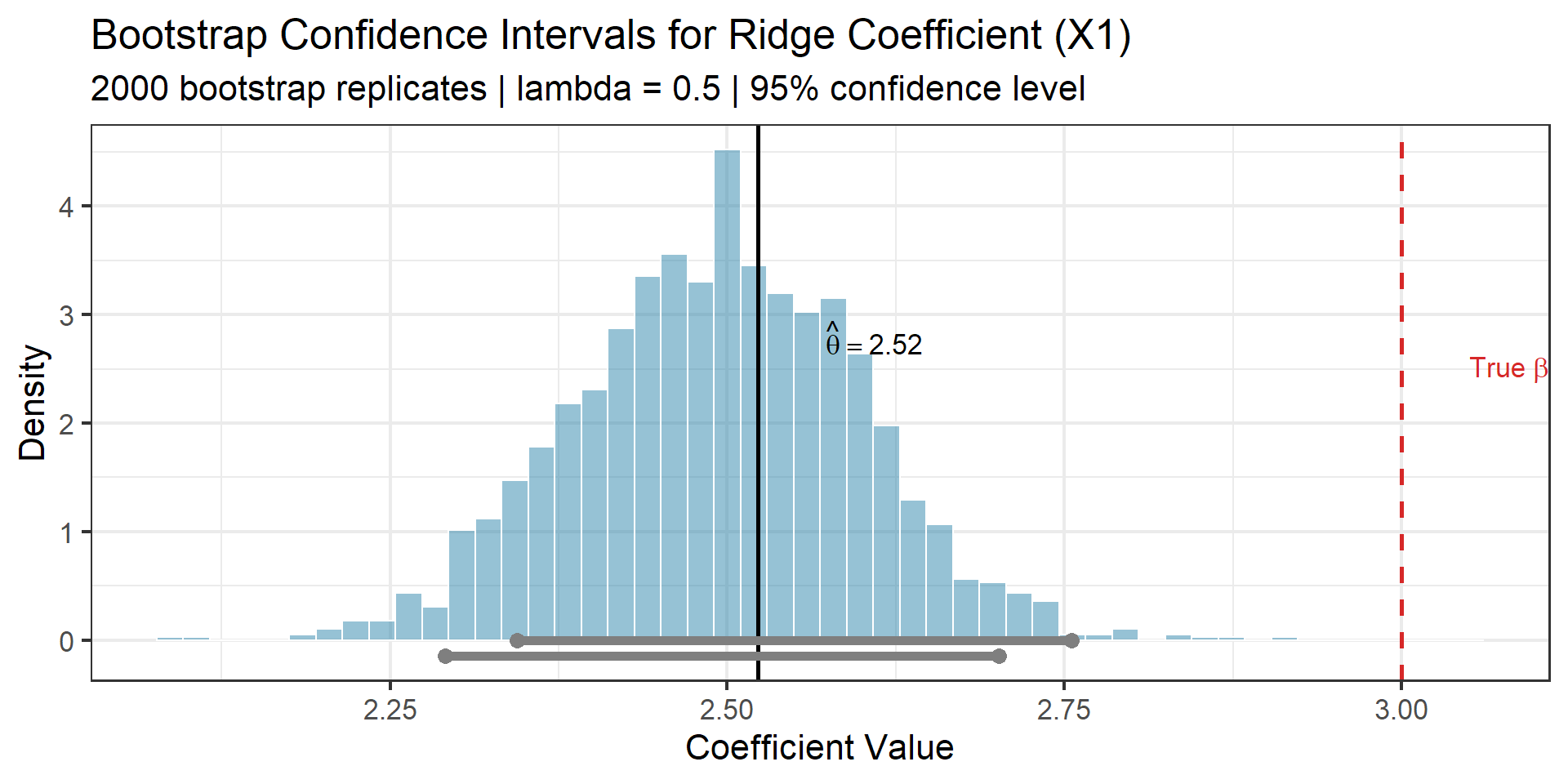
Observe
Both intervals contain the true value \(\beta_1 = 3\), but the Ridge point estimate \(\hat{\theta}\) is biased below it. The bootstrap honestly reflects this bias — the distribution is centered at the biased estimate, not the truth. This is a feature, not a bug: bootstrap intervals for shrinkage estimators correctly account for the bias-variance trade-off.
Bootstrap → Bagging
Bagging (Bootstrap AGGregatING) is literally the bootstrap applied to prediction: fit \(B\) models on bootstrap samples, average predictions. This reduces variance by a factor related to the correlation between bootstrap replicates. We will make this precise in Week 6.
Conformal Demo: Heteroskedastic Data
set.seed(577)
n <- 500
x <- runif(n, 0, 5)
y <- sin(2 * x) + rnorm(n, sd = 0.2 + 0.3 * x)

# Split into fit / calibrate / test
fit_idx <- 1:200; cal_idx <- 201:400; test_idx <- 401:500

# Fit model on training
df_fit <- data.frame(x = x[fit_idx], y = y[fit_idx])
fit <- lm(y ~ poly(x, 5), data = df_fit)

# Calibration scores
cal_pred <- predict(fit, newdata = data.frame(x = x[cal_idx]))
cal_scores <- abs(y[cal_idx] - cal_pred)

# Conformal quantile (90% coverage)
alpha <- 0.10
n_cal <- length(cal_idx)
q_level <- ceiling((1 - alpha) * (n_cal + 1)) / n_cal
qhat <- quantile(cal_scores, probs = min(q_level, 1), type = 1)

# Test predictions and intervals
test_pred <- predict(fit, newdata = data.frame(x = x[test_idx]))

# Also compute parametric intervals
pred_se <- predict(fit, newdata = data.frame(x = x[test_idx]), se.fit = TRUE)
param_margin <- qt(1 - alpha/2, df = fit$df.residual) *
  sqrt(pred_se$se.fit^2 + summary(fit)$sigma^2)

# Empirical coverage
conformal_coverage <- mean(y[test_idx] >= test_pred - qhat &
                            y[test_idx] <= test_pred + qhat)
param_coverage <- mean(y[test_idx] >= test_pred - param_margin &
                        y[test_idx] <= test_pred + param_margin)

test_df <- tibble(
  x = x[test_idx], y = y[test_idx],
  pred = test_pred,
  conf_lo = test_pred - qhat, conf_hi = test_pred + qhat,
  param_lo = test_pred - param_margin, param_hi = test_pred + param_margin
)

p_plot <- ggplot(test_df, aes(x = x)) +
  # Conformal bands
  geom_ribbon(aes(ymin = conf_lo, ymax = conf_hi), fill = colors["blue"], alpha = 0.25) +
  # Parametric bands
  geom_ribbon(aes(ymin = param_lo, ymax = param_hi), fill = colors["red"], alpha = 0.15) +
  # Data and prediction
  geom_point(aes(y = y), size = 1.5, alpha = 0.6) +
  geom_line(aes(y = pred), color = "black", linewidth = 1) +
  annotate("text", x = 0.3, y = 3.5,
           label = paste0("Conformal (", round(100*conformal_coverage), "% coverage)"),
           color = colors["blue"], size = 4.5, hjust = 0, fontface = "bold") +
  annotate("text", x = 0.3, y = 3.0,
           label = paste0("Parametric (", round(100*param_coverage), "% coverage)"),
           color = colors["red"], size = 4.5, hjust = 0, fontface = "bold") +
  labs(title = "Split Conformal vs Parametric Prediction Intervals",
       subtitle = "Heteroskedastic data: variance increases with x | Target: 90% coverage",
       x = "x", y = "y") +
  theme_bw(base_size = 16)

ggsave(file.path(fig_dir, "04_conformal_demo.png"), p_plot, width = 12, height = 5.5, dpi = 150)
p_plot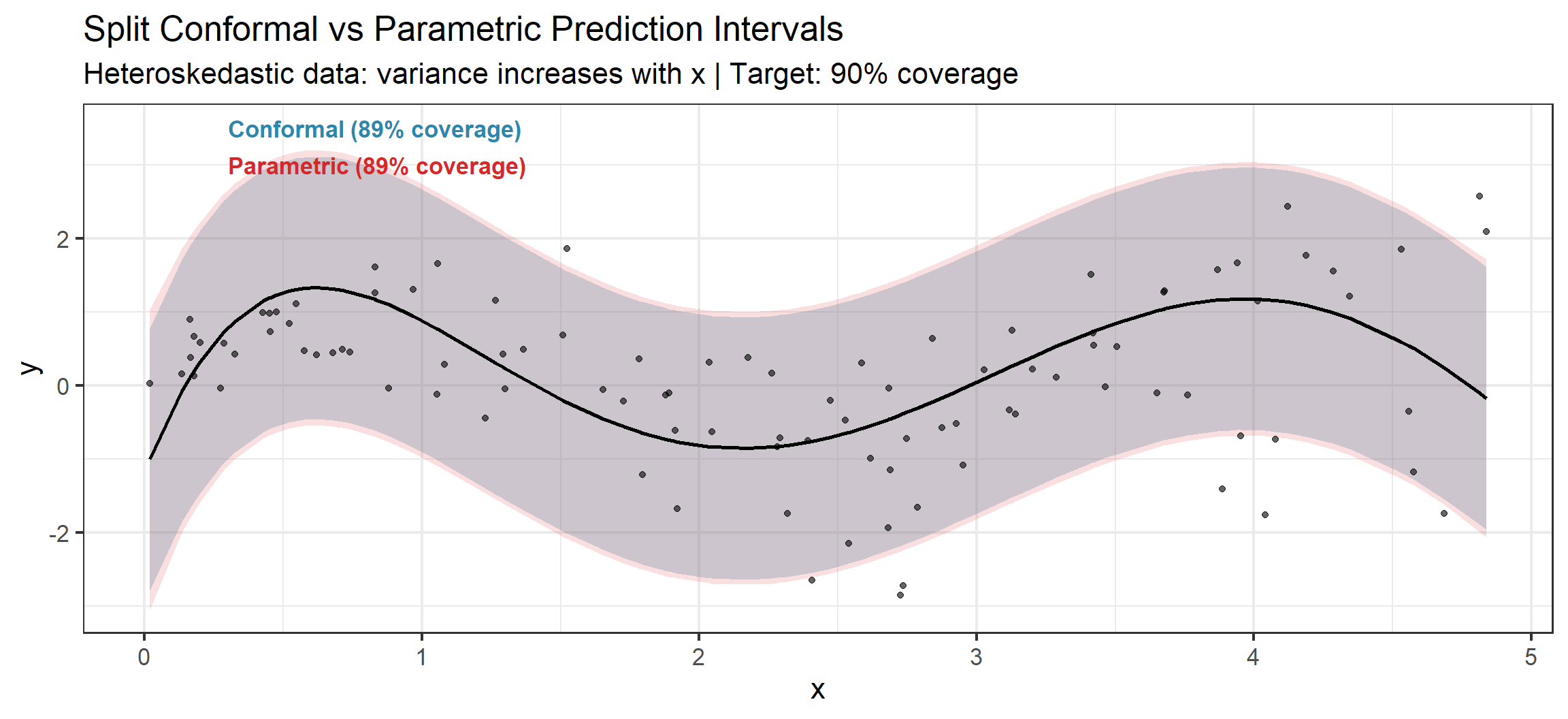
Notice the Difference
Conformal bands have constant width (since we used absolute residual scores). They are too wide on the left and too narrow on the right. Using normalized scores \(|Y - \hat{f}(X)| / \hat{\sigma}(X)\) would produce adaptive-width bands that better match the heteroskedasticity.
The Decision Framework
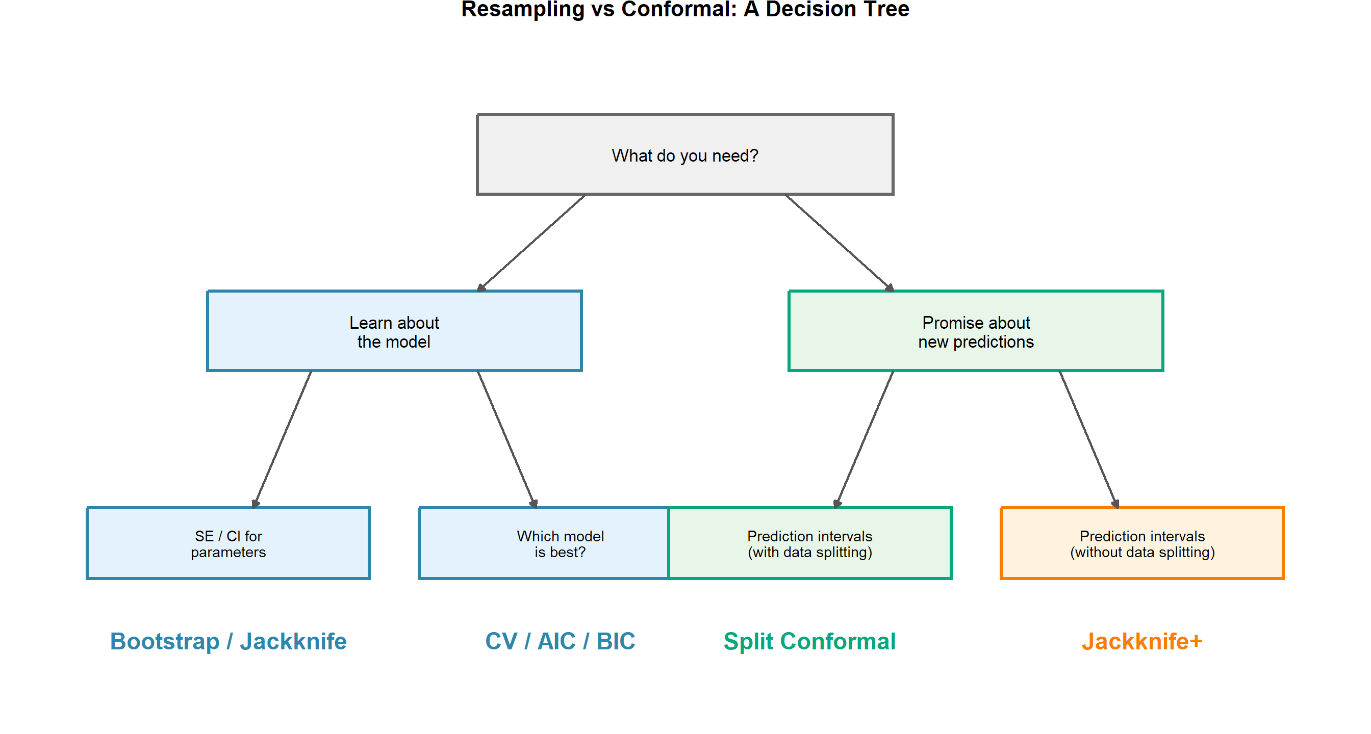
In Practice: These Paths Connect
You often use both sides sequentially. Use CV/AIC/BIC to choose your model, then wrap the chosen model in split conformal to get prediction intervals with coverage guarantees. The tree shows which tool answers which question — not that you must pick only one.