Week 6: Classification — Generative vs Discriminative

Stat 577 — Statistical Learning Theory

Soumojit Das

Spring 2026

The Classification Problem

From Regression to Classification

In regression, the response \(Y\) is continuous. Now \(Y\) takes values in a finite set \(\{1, 2, \ldots, K\}\).

Can we just use linear regression?

For \(K = 2\), code the response as 0/1 and fit \(\hat{Y} = \hat{\beta}_0 + \hat{\boldsymbol{\beta}}^T\mathbf{x}\).

Two problems:

• For \(K > 2\), any numeric coding (1, 2, 3, …) implies an ordering that may not exist
• For \(K = 2\), predicted values \(\hat{Y}\) can fall outside \([0, 1]\) — they are not valid probabilities

We need models that produce proper probability estimates.

Why Not Linear Regression? — A Demonstration

set.seed(577)
n <- 200
balance <- sort(runif(n, 0, 2500))
prob_true <- plogis(-6 + 0.004 * balance)
default <- rbinom(n, 1, prob_true)

df <- tibble(Balance = balance, Default = default)

# Fit linear regression (wrong!) and logistic regression (right)
lm_fit <- lm(Default ~ Balance, data = df)
glm_fit <- glm(Default ~ Balance, data = df, family = binomial)

pred_df <- tibble(
  Balance = seq(0, 2500, length.out = 300),
  Linear = predict(lm_fit, newdata = tibble(Balance = seq(0, 2500, length.out = 300))),
  Logistic = predict(glm_fit, newdata = tibble(Balance = seq(0, 2500, length.out = 300)),
                     type = "response")
) |> pivot_longer(-Balance, names_to = "Method", values_to = "Probability")

p <- ggplot() +
  geom_point(data = df, aes(x = Balance, y = Default), alpha = 0.3, size = 2) +
  geom_line(data = pred_df, aes(x = Balance, y = Probability, color = Method),
            linewidth = 1.3) +
  geom_hline(yintercept = c(0, 1), linetype = "dashed", alpha = 0.4) +
  scale_color_manual(values = c("Linear" = clr("red"), "Logistic" = clr("blue"))) +
  labs(title = "Why Not Linear Regression for Classification?",
       subtitle = "Linear regression produces probability estimates outside [0, 1]",
       x = "Balance", y = "P(Default)") +
  theme_bw(base_size = 16) +
  theme(legend.position = "bottom")

ggsave(file.path(fig_dir, "01_why_not_linear_regression.png"), p,
       width = 10, height = 5, dpi = 150)
p

The Bayes Classifier

Recall from Week 1: under 0-1 loss, the optimal predictor assigns each \(\mathbf{x}\) to the class with highest posterior probability.

The Bayes Classifier

\[\hat{Y}(\mathbf{x}) = \arg\max_k \; P(Y = k \mid \mathbf{X} = \mathbf{x})\]

The Bayes error rate — the irreducible error for classification — is:

\[R^* = 1 - E\!\left[\max_k P(Y = k \mid \mathbf{X})\right]\]

No classifier can do better than this. Every method we study today is an attempt to estimate the Bayes classifier from data.

The question is: how do we estimate \(P(Y = k \mid \mathbf{X} = \mathbf{x})\)?

Two fundamentally different strategies.

Two Philosophies

Generative Approach

Model the joint distribution:

\[P(\mathbf{X}, Y) = P(\mathbf{X} \mid Y) \cdot P(Y)\]

Then use Bayes’ theorem to recover \(P(Y \mid \mathbf{X})\).

Must specify:

• Class-conditional densities \(f_k(\mathbf{x}) = P(\mathbf{X} = \mathbf{x} \mid Y = k)\)
• Prior probabilities \(\pi_k = P(Y = k)\)

Examples: LDA, QDA, Naive Bayes

Discriminative Approach

Model \(P(Y \mid \mathbf{X})\) directly.

\[\log \frac{P(Y = 1 \mid \mathbf{x})}{P(Y = 0 \mid \mathbf{x})} = \beta_0 + \boldsymbol{\beta}^T\mathbf{x}\]

No need to specify how \(\mathbf{X}\) is distributed.

Must specify:

• Functional form of \(P(Y \mid \mathbf{X})\)

Examples: Logistic regression, SVM

The Punchline of Today’s Lecture

For the Gaussian case, both approaches lead to the SAME linear decision boundary — but they estimate it differently, with different strengths. Understanding when and why each wins is the core of this lecture.

The Generative Path: LDA, QDA, Naive Bayes

The Generative Setup

We model each class’s feature distribution explicitly.

Assume: The features within each class follow a multivariate Gaussian:

\[\mathbf{X} \mid Y = k \;\sim\; N(\boldsymbol{\mu}_k, \boldsymbol{\Sigma})\]

Note the shared covariance matrix \(\boldsymbol{\Sigma}\) — every class has the same spread and correlation structure. Only the means \(\boldsymbol{\mu}_k\) differ.

This is the key assumption that makes LDA linear.

Prior probabilities: \(\pi_k = P(Y = k)\), with \(\sum_{k=1}^K \pi_k = 1\).

Goal: Compute the posterior \(P(Y = k \mid \mathbf{X} = \mathbf{x})\) via Bayes’ theorem and classify to the most probable class.

Applying Bayes’ Theorem

By Bayes’ rule, the posterior probability of class \(k\) is:

\[P(Y = k \mid \mathbf{X} = \mathbf{x}) = \frac{\pi_k \, f_k(\mathbf{x})}{\sum_{\ell=1}^K \pi_\ell \, f_\ell(\mathbf{x})}\]

where the class-conditional density under our Gaussian assumption is:

\[f_k(\mathbf{x}) = \frac{1}{(2\pi)^{p/2}|\boldsymbol{\Sigma}|^{1/2}} \exp\!\left(-\frac{1}{2}(\mathbf{x} - \boldsymbol{\mu}_k)^T \boldsymbol{\Sigma}^{-1}(\mathbf{x} - \boldsymbol{\mu}_k)\right)\]

The denominator \(\sum_\ell \pi_\ell f_\ell(\mathbf{x})\) is the marginal density of \(\mathbf{X}\) — it does not depend on \(k\).

To classify, we only need to compare \(\pi_k f_k(\mathbf{x})\) across classes. Taking logarithms makes this tractable.

The Cancellation That Makes It Linear

Take the log-posterior (dropping the denominator \(\sum_\ell \pi_\ell f_\ell(\mathbf{x})\), which depends on \(\mathbf{x}\) but not on \(k\)):

\[\log P(Y = k \mid \mathbf{x}) \;=\; \log \pi_k + \log f_k(\mathbf{x}) + \text{const}(\mathbf{x})\]

Expand the quadratic form inside \(\log f_k\):

\[-\frac{1}{2}(\mathbf{x} - \boldsymbol{\mu}_k)^T \boldsymbol{\Sigma}^{-1}(\mathbf{x} - \boldsymbol{\mu}_k) = \underbrace{-\frac{1}{2}\mathbf{x}^T\boldsymbol{\Sigma}^{-1}\mathbf{x}}_{\text{same for all } k} + \mathbf{x}^T\boldsymbol{\Sigma}^{-1}\boldsymbol{\mu}_k - \frac{1}{2}\boldsymbol{\mu}_k^T\boldsymbol{\Sigma}^{-1}\boldsymbol{\mu}_k\]

The Key Cancellation

Because all classes share the same \(\boldsymbol{\Sigma}\), the quadratic term \(-\frac{1}{2}\mathbf{x}^T\boldsymbol{\Sigma}^{-1}\mathbf{x}\) is identical for every class. When we compare \(\delta_k(\mathbf{x})\) vs \(\delta_\ell(\mathbf{x})\), this term cancels.

This is WHY the discriminant function is linear in \(\mathbf{x}\).

Linear Discriminant Functions

After the cancellation, what remains defines the linear discriminant function:

LDA Discriminant Function

\[\delta_k(\mathbf{x}) = \mathbf{x}^T \boldsymbol{\Sigma}^{-1} \boldsymbol{\mu}_k - \frac{1}{2}\boldsymbol{\mu}_k^T \boldsymbol{\Sigma}^{-1} \boldsymbol{\mu}_k + \log \pi_k\]

Classification rule: \(\hat{Y}(\mathbf{x}) = \arg\max_k \; \delta_k(\mathbf{x})\)

This is linear in \(\mathbf{x}\) — hence “Linear Discriminant Analysis.”

Reading the discriminant function:

• \(\mathbf{x}^T \boldsymbol{\Sigma}^{-1} \boldsymbol{\mu}_k\): how well \(\mathbf{x}\) aligns with class \(k\)’s mean (Mahalanobis inner product)
• \(-\frac{1}{2}\boldsymbol{\mu}_k^T \boldsymbol{\Sigma}^{-1} \boldsymbol{\mu}_k\): a centering correction (penalizes classes with means far from the origin)
• \(\log \pi_k\): the prior — rare classes start with a disadvantage

Decision Boundaries

For two classes, the decision boundary is where \(\delta_1(\mathbf{x}) = \delta_2(\mathbf{x})\):

\[\mathbf{x}^T \boldsymbol{\Sigma}^{-1}(\boldsymbol{\mu}_1 - \boldsymbol{\mu}_2) = \frac{1}{2}(\boldsymbol{\mu}_1^T\boldsymbol{\Sigma}^{-1}\boldsymbol{\mu}_1 - \boldsymbol{\mu}_2^T\boldsymbol{\Sigma}^{-1}\boldsymbol{\mu}_2) - \log\frac{\pi_1}{\pi_2}\]

This is a hyperplane in feature space — a linear equation in \(\mathbf{x}\).

The optimal projection direction for two classes is:

\[\mathbf{w} = \boldsymbol{\Sigma}^{-1}(\boldsymbol{\mu}_1 - \boldsymbol{\mu}_2)\]

Week 2 callback: just like the linear regression decision surface, this is a hyperplane. But now it separates classes rather than partitioning the regression space.

LDA Decision Boundary — Visualization

set.seed(577)
n_per_class <- 150

# Shared covariance with correlation
Sigma <- matrix(c(1, 0.5, 0.5, 1.5), 2, 2)
mu1 <- c(-1, -1)
mu2 <- c(1.5, 1)

X1 <- mvrnorm(n_per_class, mu1, Sigma)
X2 <- mvrnorm(n_per_class, mu2, Sigma)

df_lda <- tibble(
  x1 = c(X1[,1], X2[,1]),
  x2 = c(X1[,2], X2[,2]),
  class = factor(rep(c("Class 1", "Class 2"), each = n_per_class))
)

# Fit LDA
lda_fit <- lda(class ~ x1 + x2, data = df_lda)

# Create decision boundary grid
grid <- expand.grid(
  x1 = seq(min(df_lda$x1) - 1, max(df_lda$x1) + 1, length.out = 200),
  x2 = seq(min(df_lda$x2) - 1, max(df_lda$x2) + 1, length.out = 200)
)
grid$pred <- predict(lda_fit, grid)$class

p <- ggplot() +
  geom_tile(data = grid, aes(x = x1, y = x2, fill = pred), alpha = 0.15) +
  geom_point(data = df_lda, aes(x = x1, y = x2, color = class), size = 2, alpha = 0.7) +
  geom_point(aes(x = mu1[1], y = mu1[2]), shape = 4, size = 5, stroke = 2,
             color = "black") +
  geom_point(aes(x = mu2[1], y = mu2[2]), shape = 4, size = 5, stroke = 2,
             color = "black") +
  scale_color_manual(values = c("Class 1" = clr("blue"),
                                "Class 2" = clr("red"))) +
  scale_fill_manual(values = c("Class 1" = clr("blue"),
                               "Class 2" = clr("red"))) +
  labs(title = "LDA Decision Boundary (Shared Covariance)",
       subtitle = "x marks class means | Linear boundary from equal Sigma assumption",
       x = expression(X[1]), y = expression(X[2]), color = "True Class") +
  guides(fill = "none") +
  theme_bw(base_size = 16) +
  theme(legend.position = "bottom")

ggsave(file.path(fig_dir, "02_lda_decision_boundary.png"), p,
       width = 10, height = 6, dpi = 150)
p

Plug-in Estimates from Data

In practice, we replace population quantities with sample estimates:

Prior probabilities: \[\hat{\pi}_k = \frac{n_k}{n}\]

Class means: \[\hat{\boldsymbol{\mu}}_k = \frac{1}{n_k}\sum_{i:\, y_i = k} \mathbf{x}_i\]

Pooled covariance (weighted average of within-class covariances): \[\hat{\boldsymbol{\Sigma}} = \frac{1}{n - K}\sum_{k=1}^K \sum_{i:\, y_i = k} (\mathbf{x}_i - \hat{\boldsymbol{\mu}}_k)(\mathbf{x}_i - \hat{\boldsymbol{\mu}}_k)^T\]

Plug these into \(\delta_k(\mathbf{x})\) and classify.

Under the Gaussian equal-covariance assumption, LDA is the optimal classifier — it is the plug-in Bayes rule.

How Prior Probabilities Shift the Boundary

The prior \(\pi_k\) is not just a book-keeping term — it actively shapes the decision boundary.

At \(\pi_1 = 0.5\) (equal priors), the boundary bisects the means. As \(\pi_1\) decreases, the boundary shifts toward Class 1 — a rarer class needs stronger evidence to be claimed. The \(\log\pi_k\) term in \(\delta_k(\mathbf{x})\) drives this shift.

Fisher’s Linear Discriminant (1936)

Fisher’s Insight: Same Direction, Different Motivation

Fisher arrived at the same discriminant direction \(\boldsymbol{\Sigma}^{-1}(\boldsymbol{\mu}_1 - \boldsymbol{\mu}_2)\) without assuming Gaussianity.

His approach: find the projection \(\mathbf{w}\) that maximizes the ratio of between-class to within-class variance — the Rayleigh quotient:

\[J(\mathbf{w}) = \frac{\mathbf{w}^T \mathbf{S}_B \, \mathbf{w}}{\mathbf{w}^T \mathbf{S}_W \, \mathbf{w}}\]

For two classes: \(\mathbf{S}_B = (\bar{\mathbf{x}}_1 - \bar{\mathbf{x}}_2)(\bar{\mathbf{x}}_1 - \bar{\mathbf{x}}_2)^T\) and \(\mathbf{S}_W\) is the pooled within-class scatter.

Solution: \(\mathbf{w} \propto \mathbf{S}_W^{-1}(\bar{\mathbf{x}}_1 - \bar{\mathbf{x}}_2)\)

For \(K > 2\) classes, the between-class scatter generalizes to \(\mathbf{S}_B = \sum_{k=1}^K n_k (\bar{\mathbf{x}}_k - \bar{\mathbf{x}})(\bar{\mathbf{x}}_k - \bar{\mathbf{x}})^T\), and \(\mathbf{S}_B\) has rank at most \(K - 1\). The eigenvectors of \(\mathbf{S}_W^{-1}\mathbf{S}_B\) give at most \(K - 1\) discriminant directions — the coordinates of Fisher’s reduced subspace.

The fact that two completely different motivations — probabilistic (Gaussian + Bayes) and geometric (maximize class separation) — give the same direction is remarkable. This convergence from different starting points is a hallmark of a fundamental result.

LDA as Nearest-Centroid in “Whitened” Space

There is a deeper geometric way to see why LDA works.

“Whitening” (also called sphering) means transforming the data so that the covariance becomes the identity matrix — all variables are uncorrelated and have unit variance. The name comes from the analogy with white noise, which has a flat (identity) power spectrum.

Step 1 — Whiten the data. Apply the transformation \(\mathbf{z} = \boldsymbol{\Sigma}^{-1/2}\mathbf{x}\), so that \(\mathbf{Z} \mid Y = k \;\sim\; N(\boldsymbol{\Sigma}^{-1/2}\boldsymbol{\mu}_k,\; \mathbf{I})\).

In the whitened space, both classes have identity covariance — they are spherical clouds.

Step 2 — Classify to nearest mean. With identity covariance, the Mahalanobis distance reduces to Euclidean distance. The optimal rule is: assign \(\mathbf{z}\) to the class whose transformed mean \(\boldsymbol{\Sigma}^{-1/2}\boldsymbol{\mu}_k\) is closest.

The decision boundary in the whitened space is the perpendicular bisector of the segment joining \(\boldsymbol{\Sigma}^{-1/2}\boldsymbol{\mu}_1\) and \(\boldsymbol{\Sigma}^{-1/2}\boldsymbol{\mu}_2\) — the simplest possible boundary.

The Sphering Interpretation

LDA = sphere the data with \(\boldsymbol{\Sigma}^{-1/2}\), then apply nearest-centroid classification in the sphered space.

All the complexity of LDA — the inverse covariance, the quadratic form in \(\delta_k\) — is just the algebra of doing Euclidean nearest-centroid after a change of coordinates. The direction \(\boldsymbol{\Sigma}^{-1}(\boldsymbol{\mu}_1 - \boldsymbol{\mu}_2)\) is simply the line connecting the two means, mapped back to the original coordinate system.

Look familiar? If you squint, LDA is supervised \(K\)-means after whitening — both assign to the nearest centroid in Euclidean space. The difference: LDA knows the labels and estimates centroids from them; \(K\)-means discovers centroids without labels. We will revisit this connection when we cover unsupervised learning.

QDA: Relaxing Equal Covariance

Now each class gets its own covariance matrix:

\[\mathbf{X} \mid Y = k \;\sim\; N(\boldsymbol{\mu}_k, \boldsymbol{\Sigma}_k)\]

The quadratic term \(-\frac{1}{2}\mathbf{x}^T\boldsymbol{\Sigma}_k^{-1}\mathbf{x}\) now depends on \(k\) — it does NOT cancel!

The discriminant functions become quadratic in \(\mathbf{x}\):

QDA Discriminant Function

\[\delta_k(\mathbf{x}) = -\frac{1}{2}\log|\boldsymbol{\Sigma}_k| - \frac{1}{2}(\mathbf{x} - \boldsymbol{\mu}_k)^T\boldsymbol{\Sigma}_k^{-1}(\mathbf{x} - \boldsymbol{\mu}_k) + \log \pi_k\]

Decision boundaries are now quadratic surfaces — conic sections (ellipses, parabolas, hyperbolas) in 2D.

More flexible than LDA, but at a cost.

Shared vs Separate Covariance: The Geometric Story

Left: When \(\boldsymbol{\Sigma}_1 = \boldsymbol{\Sigma}_2\), the density ellipses have identical shapes — only their centers differ. The boundary is a straight line.

Right: When \(\boldsymbol{\Sigma}_1 \neq \boldsymbol{\Sigma}_2\), one class is circular while the other is elongated. No straight line can separate them well — the boundary must bend.

LDA vs QDA: The Bias-Variance Tradeoff

Parameter count comparison:

Method	Parameters to estimate
LDA	\(Kp + p(p+1)/2 + (K-1)\)
QDA	\(Kp + K \cdot p(p+1)/2 + (K-1)\)

(The \((K-1)\) term counts the free prior probabilities; it is negligible relative to the covariance terms.)

Concrete example: With \(p = 50\) features and \(K = 3\) classes:

• LDA: \(\approx 1{,}427\) parameters (means + shared covariance + priors)
• QDA: \(\approx 3{,}977\) parameters (means + \(K\) covariances + priors)

QDA and the Curse of Dimensionality

QDA requires estimating \(K\) separate \(p \times p\) covariance matrices. With limited data, these estimates are noisy and QDA can overfit badly.

Week 1 callback: this is the bias-variance tradeoff in action. QDA has less bias (more flexible boundaries) but more variance (more parameters to estimate). When \(n\) is small relative to \(p\), LDA wins despite its stronger assumptions.

Naive Bayes: Independence as Extreme Regularization

Assumption: Features are conditionally independent given the class:

\[f_k(\mathbf{x}) = \prod_{j=1}^p f_{kj}(x_j)\]

This is extreme regularization — it forces \(\boldsymbol{\Sigma}_k\) to be diagonal.

• Gaussian Naive Bayes with shared variances = LDA with a diagonal covariance matrix
• Parameter count drops from \(O(p^2)\) to \(O(p)\)

Works surprisingly well even when the independence assumption is clearly violated.

Naive Bayes as Regularization

Both Naive Bayes and the lasso impose hard structural zeros — lasso in the coefficient vector, Naive Bayes in the off-diagonal entries of \(\boldsymbol{\Sigma}_k\) — trading bias for dramatic variance reduction. In high dimensions (\(p \gg n\)), this can be a winning trade.

The independence assumption is almost always wrong. But the parameters it produces can be more stable than those from a correctly specified but poorly estimated full-covariance model. The analogy is not exact — lasso zeros are data-adaptive while NB zeros are structural — but the statistical logic is the same: when you cannot afford to estimate everything, force most of it to zero.

We have built classifiers by modeling \(P(\mathbf{X} \mid Y)\) — the generative path. Now we flip the direction: model \(P(Y \mid \mathbf{X})\) directly, and see what we gain by giving up the generative model.

The Discriminative Path: Logistic Regression

A Different Philosophy

Instead of modeling the full joint distribution \(P(\mathbf{X}, Y)\) and using Bayes’ theorem, we model \(P(Y \mid \mathbf{X})\) directly.

What we give up: We never learn how the features are distributed within each class.

What we gain: We do not need to make distributional assumptions about \(\mathbf{X}\).

If the goal is classification — predicting \(Y\) from \(\mathbf{X}\) — do we really need to know \(P(\mathbf{X} \mid Y)\)?

The discriminative philosophy says no. Model only what you need.

The Logistic Regression Model

For \(K = 2\) classes, model the log-odds as linear in \(\mathbf{x}\):

\[\log \frac{P(Y = 1 \mid \mathbf{x})}{P(Y = 0 \mid \mathbf{x})} = \beta_0 + \boldsymbol{\beta}^T\mathbf{x}\]

Equivalently, the probability of class 1 is:

\[P(Y = 1 \mid \mathbf{x}) = \frac{e^{\beta_0 + \boldsymbol{\beta}^T\mathbf{x}}}{1 + e^{\beta_0 + \boldsymbol{\beta}^T\mathbf{x}}} = \sigma(\beta_0 + \boldsymbol{\beta}^T\mathbf{x})\]

where \(\sigma(z) = 1/(1 + e^{-z})\) is the sigmoid (logistic) function.

The decision boundary \(\{\mathbf{x} : \beta_0 + \boldsymbol{\beta}^T\mathbf{x} = 0\}\) is linear — the same functional form as LDA!

What Logistic Regression Assumes (and Doesn’t)

Logistic regression makes no distributional assumption about \(\mathbf{X}\) — no Gaussianity, no particular marginal form. But it does require correct specification of the functional form: the log-odds must truly be linear in \(\mathbf{x}\). If the true log-odds are quadratic or involve interactions, a linear logistic model is misspecified. “No distributional assumption on \(\mathbf{X}\)” \(\neq\) “no assumptions at all.”

Compare with LDA: assumes \(\mathbf{X} \mid Y\) is Gaussian with shared covariance, from which linearity of the log-odds follows as a consequence. LDA makes a stronger assumption, but when it holds, that assumption does real work — it gives you the correct functional form for free.

Coefficient Interpretation

Each coefficient \(\beta_j\) has a precise interpretation:

• \(\beta_j\) = change in log-odds per unit increase in \(x_j\), holding other predictors fixed

• \(e^{\beta_j}\) = odds ratio — the multiplicative effect on odds

Example: If \(\beta_j = 0.5\), then each unit increase in \(x_j\) multiplies the odds by \(e^{0.5} \approx 1.65\) — a 65% increase in odds.

Caution: “Holding other predictors fixed” is doing a lot of work in this interpretation. With correlated predictors, the marginal effect of \(x_j\) can differ substantially from the conditional effect \(\beta_j\).

Maximum Likelihood Estimation

The likelihood for \(n\) binary observations \((y_i \in \{0, 1\})\):

\[L(\boldsymbol{\beta}) = \prod_{i=1}^n p(\mathbf{x}_i)^{y_i}\bigl(1 - p(\mathbf{x}_i)\bigr)^{1-y_i}\]

The log-likelihood:

\[\ell(\boldsymbol{\beta}) = \sum_{i=1}^n \left[y_i \log p(\mathbf{x}_i) + (1 - y_i) \log\bigl(1 - p(\mathbf{x}_i)\bigr)\right]\]

where \(p(\mathbf{x}_i) = \sigma(\beta_0 + \boldsymbol{\beta}^T\mathbf{x}_i)\).

No closed-form solution — the sigmoid makes the score equations nonlinear.

We need iterative methods.

IRLS: Logistic Regression as Iterative Weighted Least Squares

Newton-Raphson on the log-likelihood gives the update:

\[\boldsymbol{\beta}^{(t+1)} = \boldsymbol{\beta}^{(t)} + (\mathbf{X}^T\mathbf{W}\mathbf{X})^{-1}\mathbf{X}^T(\mathbf{y} - \hat{\mathbf{p}})\]

where \(\mathbf{W} = \text{diag}\bigl(\hat{p}_i(1-\hat{p}_i)\bigr)\) is a diagonal weight matrix.

Rearrange to get the IRLS form:

\[\boldsymbol{\beta}^{(t+1)} = (\mathbf{X}^T\mathbf{W}\mathbf{X})^{-1}\mathbf{X}^T\mathbf{W}\mathbf{z}\]

where \(\mathbf{z} = \mathbf{X}\boldsymbol{\beta}^{(t)} + \mathbf{W}^{-1}(\mathbf{y} - \hat{\mathbf{p}})\) is the “working response.”

IRLS = Repeatedly Fitting Weighted Linear Regressions

Each iteration of IRLS is a weighted least squares fit. The weights \(w_i = \hat{p}_i(1-\hat{p}_i)\) are largest when the model is most uncertain (\(\hat{p}_i \approx 0.5\)), giving uncertain points the most influence.

Week 2 callback: the hat matrix \(\mathbf{H} = \mathbf{X}(\mathbf{X}^T\mathbf{W}\mathbf{X})^{-1}\mathbf{X}^T\mathbf{W}\) appears again — logistic regression inherits the projection geometry of linear regression, just with adaptive weights. Note a key difference from the OLS hat matrix: this \(\mathbf{H}\) is not symmetric (since \(\mathbf{W}\) is not proportional to \(\mathbf{I}\)) and does not satisfy \(\mathbf{H}^2 = \mathbf{H}\). It maps working responses \(\mathbf{z}\) to fitted values \(\hat{\mathbf{z}}\), but it is not an orthogonal projection in the usual sense.

We have seen how to optimize — Newton-Raphson via IRLS. Now let us understand what we are optimizing, and why the negative log-likelihood is the natural loss function for classification.

Cross-Entropy Loss = KL Divergence

Consider the negative log-likelihood — the loss function we are minimizing:

\[-\ell(\boldsymbol{\beta}) = -\sum_{i=1}^n \left[y_i \log \hat{p}_i + (1 - y_i) \log(1 - \hat{p}_i)\right]\]

This is the cross-entropy loss.

Week 4 payoff. The negative log-likelihood above is the cross-entropy \(H(p, q)\) between the empirical label distribution \(p\) and the model’s predicted distribution \(q\). Now recall the decomposition from Week 4:

\[D_{\text{KL}}(p \,\|\, q) = H(p, q) - H(p)\]

The entropy of the true labels \(H(p)\) does not depend on the model parameters — it is a fixed property of the data. So minimizing the cross-entropy \(H(p, q)\) over model parameters is equivalent to minimizing \(D_{\text{KL}}(p \,\|\, q)\).

Minimizing the negative log-likelihood is exactly minimizing KL divergence from the true class distribution to the model distribution.

The Week 4 Payoff

The cross-entropy loss in logistic regression is the KL divergence \(D_{\text{KL}}(p_{\text{true}} \,\|\, p_{\text{model}})\) plus a constant. When we fit logistic regression by MLE, we are finding the model closest to truth in the information-theoretic sense.

This is NOT a coincidence — it is why MLE is the natural estimation principle for classification. The same connection drove AIC in Week 4: there, KL divergence justified penalized likelihood for model selection. Here, it justifies the loss function itself.

Multinomial Logistic Regression

For \(K > 2\) classes, use \(K - 1\) log-odds relative to a baseline class \(K\):

\[\log \frac{P(Y = k \mid \mathbf{x})}{P(Y = K \mid \mathbf{x})} = \beta_{k0} + \boldsymbol{\beta}_k^T\mathbf{x}, \qquad k = 1, \ldots, K-1\]

The probabilities are:

\[P(Y = k \mid \mathbf{x}) = \frac{e^{\beta_{k0} + \boldsymbol{\beta}_k^T\mathbf{x}}}{1 + \sum_{\ell=1}^{K-1} e^{\beta_{\ell 0} + \boldsymbol{\beta}_\ell^T\mathbf{x}}}, \qquad P(Y = K \mid \mathbf{x}) = \frac{1}{1 + \sum_{\ell=1}^{K-1} e^{\beta_{\ell 0} + \boldsymbol{\beta}_\ell^T\mathbf{x}}}\]

Decision boundaries remain hyperplanes between each pair of classes.

The choice of baseline class does not affect predictions — only the parameterization.

The Punchline: Same Boundary, Different Estimation

The Remarkable Coincidence

Two completely different starting points lead to the same model:

LDA: Start from \(P(\mathbf{X} \mid Y)\) Gaussian with shared \(\boldsymbol{\Sigma}\). Compute the log-posterior via Bayes’ theorem. Get a linear function of \(\mathbf{x}\).

Logistic Regression: Directly model \(\log\frac{P(Y=1 \mid \mathbf{x})}{P(Y=0 \mid \mathbf{x})} = \beta_0 + \boldsymbol{\beta}^T\mathbf{x}\).

Same functional form. Both give linear decision boundaries. Under the LDA model, the implied logistic regression coefficients are:

\[\boldsymbol{\beta} = \boldsymbol{\Sigma}^{-1}(\boldsymbol{\mu}_1 - \boldsymbol{\mu}_2), \qquad \beta_0 = -\tfrac{1}{2}(\boldsymbol{\mu}_1 + \boldsymbol{\mu}_2)^T\boldsymbol{\Sigma}^{-1}(\boldsymbol{\mu}_1 - \boldsymbol{\mu}_2) + \log\frac{\pi_1}{\pi_2}\]

This is what “same boundary” means concretely: if the Gaussian model is correct, the LDA parameters \((\boldsymbol{\mu}_1, \boldsymbol{\mu}_2, \boldsymbol{\Sigma}, \pi_1, \pi_2)\) determine the logistic coefficients \((\beta_0, \boldsymbol{\beta})\) exactly.

But they estimate the parameters differently, and this difference has consequences.

Joint vs Conditional Likelihood

LDA: Joint Likelihood

Maximizes: \[\prod_{i=1}^n P(\mathbf{x}_i, y_i) = \prod_{i=1}^n P(\mathbf{x}_i \mid y_i)\, P(y_i)\]

Estimates \(\boldsymbol{\mu}_k\), \(\boldsymbol{\Sigma}\), \(\pi_k\) separately, then derives the boundary from these.

Uses all the information in the data — including the marginal distribution of \(\mathbf{X}\).

Logistic: Conditional Likelihood

Maximizes: \[\prod_{i=1}^n P(y_i \mid \mathbf{x}_i)\]

Directly estimates \(\beta_0, \boldsymbol{\beta}\) — the boundary parameters.

Ignores the marginal distribution of \(\mathbf{X}\) entirely.

The joint likelihood uses more information, so LDA should be more efficient — if its assumptions hold.

But if they do not hold, the extra “information” LDA extracts from the marginal is actually misinformation.

Efron’s Efficiency Result (1975)

Efron (1975): Asymptotic Relative Efficiency of Logistic vs LDA

When the Gaussian equal-covariance assumption holds, the asymptotic relative efficiency (ARE) of logistic regression to LDA depends on the Mahalanobis distance \(\Delta^2 = (\boldsymbol{\mu}_1 - \boldsymbol{\mu}_2)^T\boldsymbol{\Sigma}^{-1}(\boldsymbol{\mu}_1 - \boldsymbol{\mu}_2)\) between the classes:

• Full overlap (\(\Delta \to 0\)): ARE \(\to 1\) — logistic loses almost nothing.
• Moderate separation: ARE \(\approx 2/3\) — logistic uses roughly two-thirds of the information LDA extracts. This is where the often-cited “one-third loss” applies.
• Well-separated classes (\(\Delta\) large): ARE \(\to 1/2\) — logistic needs about twice the sample size to match LDA’s precision.

But when the Gaussian assumption fails, LDA can be inconsistent — it converges to the wrong boundary because the “information” it extracts from the misspecified marginal \(P(\mathbf{X})\) is misinformation. Logistic regression, which never models \(P(\mathbf{X})\), converges to the best linear boundary in the KL sense regardless.

The practical implication:

• LDA’s best-case advantage is a factor-of-two efficiency gain (well-separated Gaussian classes) — meaningful but bounded
• Under misspecification, the comparison reverses qualitatively: logistic converges to a useful boundary, LDA may not
• LDA can win meaningfully when \(n\) is small and the Gaussian assumption is approximately correct

This is a recurring theme: robustness often trumps efficiency. A modest efficiency loss under ideal conditions is a small price for consistency under realistic conditions.

Ng & Jordan (2002): A Bias-Variance Story

Ng and Jordan formalized a complementary result. Generative classifiers (like Naive Bayes) converge to their asymptotic error faster — at rate \(O(1/n)\) in the number of parameters — while discriminative classifiers (like logistic regression) converge more slowly, at rate \(O(1/\sqrt{n})\).

But the asymptotic error of the discriminative classifier is lower (or equal), because it makes fewer assumptions.

The result: there exists a crossover sample size \(n^*\) below which the generative model has lower test error, and above which the discriminative model wins. This is the bias-variance tradeoff in its purest form — high bias / low variance (generative) vs. low bias / high variance (discriminative).

Head-to-Head: Three Scenarios

set.seed(577)
n_per <- 200

# Scenario 1: Gaussian with shared Sigma (LDA should win)
Sigma_shared <- matrix(c(1, 0.3, 0.3, 1), 2, 2)
g1_c1 <- mvrnorm(n_per, c(-1, -0.5), Sigma_shared)
g1_c2 <- mvrnorm(n_per, c(1, 0.5), Sigma_shared)
df_gauss <- tibble(x1 = c(g1_c1[,1], g1_c2[,1]),
                   x2 = c(g1_c1[,2], g1_c2[,2]),
                   class = factor(rep(0:1, each = n_per)))

# Scenario 2: Different covariances (QDA should win)
g2_c1 <- mvrnorm(n_per, c(-1, 0), matrix(c(1, 0, 0, 0.3), 2, 2))
g2_c2 <- mvrnorm(n_per, c(1, 0), matrix(c(0.3, 0, 0, 1), 2, 2))
df_diffcov <- tibble(x1 = c(g2_c1[,1], g2_c2[,1]),
                     x2 = c(g2_c1[,2], g2_c2[,2]),
                     class = factor(rep(0:1, each = n_per)))

# Scenario 3: Contaminated Gaussian (logistic should win)
# 90% clean Gaussian + 10% from 25x inflated covariance
n_clean <- round(0.9 * n_per)
n_outlier <- n_per - n_clean
contam_c1 <- rbind(
  mvrnorm(n_clean, c(-1, -0.5), Sigma_shared),
  mvrnorm(n_outlier, c(-1, -0.5), 25 * Sigma_shared)
)
contam_c2 <- rbind(
  mvrnorm(n_clean, c(1, 0.5), Sigma_shared),
  mvrnorm(n_outlier, c(1, 0.5), 25 * Sigma_shared)
)
df_contam <- tibble(x1 = c(contam_c1[,1], contam_c2[,1]),
                    x2 = c(contam_c1[,2], contam_c2[,2]),
                    class = factor(rep(0:1, each = n_per)))

# Function to compute decision boundaries for all three methods
plot_boundaries <- function(df, title_text, subtitle_text = NULL) {
  grid <- expand.grid(
    x1 = seq(min(df$x1) - 0.5, max(df$x1) + 0.5, length.out = 150),
    x2 = seq(min(df$x2) - 0.5, max(df$x2) + 0.5, length.out = 150)
  )

  # Factor levels "0" < "1", so glm models P(class = "1") and
  # lda posterior[,2] is also P(class = "1") --- they align correctly.
  lda_fit <- lda(class ~ x1 + x2, data = df)
  qda_fit <- qda(class ~ x1 + x2, data = df)
  glm_fit <- glm(class ~ x1 + x2, data = df, family = binomial)

  grid$lda_prob <- predict(lda_fit, grid)$posterior[,2]
  grid$qda_prob <- predict(qda_fit, grid)$posterior[,2]
  grid$logistic_prob <- predict(glm_fit, grid, type = "response")

  ggplot(df, aes(x = x1, y = x2)) +
    geom_point(aes(color = class), alpha = 0.5, size = 1.5) +
    geom_contour(data = grid, aes(z = lda_prob), breaks = 0.5,
                 color = colors["blue"], linewidth = 1.2, linetype = "solid") +
    geom_contour(data = grid, aes(z = qda_prob), breaks = 0.5,
                 color = colors["red"], linewidth = 1.2, linetype = "dashed") +
    geom_contour(data = grid, aes(z = logistic_prob), breaks = 0.5,
                 color = colors["green"], linewidth = 1.2, linetype = "dotdash") +
    scale_color_manual(values = c("0" = clr("blue"), "1" = clr("red")),
                       labels = c("Class 0", "Class 1")) +
    labs(title = title_text, subtitle = subtitle_text,
         x = expression(X[1]), y = expression(X[2]),
         color = "True Class") +
    theme_bw(base_size = 14) +
    theme(legend.position = "bottom")
}

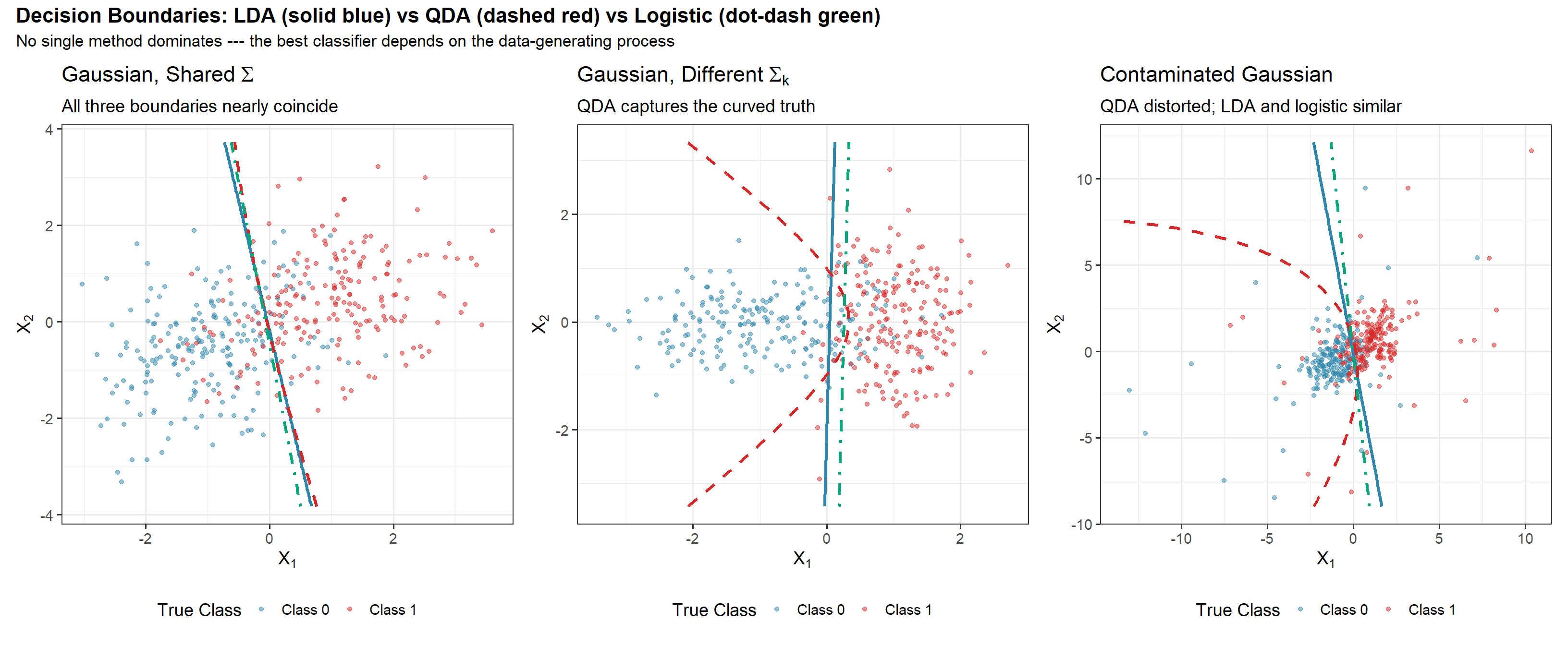
p1 <- plot_boundaries(df_gauss,
  title_text = expression("Gaussian, Shared" ~ Sigma),
  subtitle_text = "All three boundaries nearly coincide")
p2 <- plot_boundaries(df_diffcov,
  title_text = expression("Gaussian, Different" ~ Sigma[k]),
  subtitle_text = "QDA captures the curved truth")
p3 <- plot_boundaries(df_contam,
  title_text = "Contaminated Gaussian",
  subtitle_text = "QDA distorted; LDA and logistic similar")

p_combined <- p1 + p2 + p3 +
  plot_annotation(
    title = "Decision Boundaries: LDA (solid blue) vs QDA (dashed red) vs Logistic (dot-dash green)",
    subtitle = "No single method dominates --- the best classifier depends on the data-generating process",
    theme = theme(plot.title = element_text(size = 16, face = "bold"),
                  plot.subtitle = element_text(size = 13))
  )

ggsave(file.path(fig_dir, "03_lda_qda_logistic_comparison.png"), p_combined,
       width = 16, height = 6, dpi = 150)
p_combined

Reading the Three Scenarios

Left panel — Gaussian, shared \(\boldsymbol{\Sigma}\):

• LDA’s assumptions are exactly satisfied, so it achieves the Bayes-optimal boundary.
• But all three methods produce nearly identical boundaries — when the model is correct, there is little to gain or lose.

Center panel — Gaussian, different \(\boldsymbol{\Sigma}_k\):

• LDA’s equal-covariance assumption is violated. Its linear boundary cannot capture the true shape.
• QDA’s quadratic boundary adapts to the different spreads.

Right panel — Contaminated Gaussian (10% outliers from \(25\boldsymbol{\Sigma}\)):

• QDA is visibly distorted — it tries to model the contaminated distribution with a single Gaussian per class.
• LDA and logistic regression both produce reasonable linear boundaries. Logistic is slightly more robust (it never models \(P(\mathbf{X} \mid Y)\)), but visually the difference is subtle.

What the Classifier Sees: Posterior Probability Landscapes

The decision boundary is just the 0.5 contour. But each method produces a full probability surface — and those surfaces differ dramatically.

LDA’s probability contours are parallel straight lines (linear log-odds). QDA’s contours are curved — it captures the asymmetry in class spreads. Logistic regression also produces straight contours, but without assuming Gaussianity.

Explore This: Interactive Posterior Surface

Rotate and zoom to explore! The sigmoid “cliff” at the decision boundary shows how the probability transitions from 0 to 1. The steepness of the cliff reflects model confidence.

When to Use Which? — A Decision Framework

Condition	Recommended Method
Gaussian features, shared \(\boldsymbol{\Sigma}\), moderate \(n\)	LDA
Gaussian features, different \(\boldsymbol{\Sigma}_k\), large \(n\)	QDA
Non-Gaussian features, moderate \(p\)	Logistic regression
High \(p\), limited \(n\)	LDA or Naive Bayes (regularization helps)
Need well-calibrated probabilities	Logistic regression
Complex nonlinear boundaries	k-NN, trees, SVMs (Week 7+)

A Practical Pathology: Complete Separation

Before we move to regularized models, one important warning about logistic regression.

When the two classes are perfectly separable in feature space — there exists a hyperplane with zero training errors — the MLE for logistic regression does not exist. The likelihood can be made arbitrarily large by pushing \(\|\boldsymbol{\beta}\| \to \infty\), driving the predicted probabilities toward 0 and 1.

This is not a theoretical curiosity:

• It happens routinely when \(p > n\) (more features than observations)
• It happens with rare events (e.g., fraud detection with very few positive cases)
• The fitted coefficients and standard errors become numerically unstable long before true non-convergence

Complete Separation Motivates Regularization

Complete separation is one of the strongest practical motivations for regularized logistic regression. Adding a ridge or lasso penalty to the log-likelihood ensures a finite, unique solution even when the classes are perfectly separable. The penalty prevents \(\|\boldsymbol{\beta}\| \to \infty\) by making large coefficients costly.

This is the bridge to the next section.

The Modern Classification Pipeline

Week 3 Callback: Regularized Logistic Regression

glmnet for classification: same interface, just family = "binomial".

The penalized log-likelihood:

\[\max_{\boldsymbol{\beta}} \left\{\ell(\boldsymbol{\beta}) - \lambda\, P_{\text{EN}}(\boldsymbol{\beta})\right\}\]

where \(P_{\text{EN}}\) is the elastic net penalty from Week 3 (the alpha parameter in glmnet controls the \(\ell_1\)/\(\ell_2\) balance):

• alpha = 1: Lasso (variable selection + classification)
• alpha = 0: Ridge (shrinkage, no selection)
• 0 < alpha < 1: Elastic net

Same Tool, New Task

glmnet handles regression AND classification with the same interface. The only change is family = "binomial". Regularization paths, cross-validation, and the 1-SE rule all carry over directly.

The lasso penalty does variable selection and classification simultaneously — identifying which features matter for the decision boundary.

Code Demo: cv.glmnet for Classification

set.seed(577)
n <- 400; p <- 20
X <- matrix(rnorm(n * p), n, p)
beta_true <- c(1.5, -1, 0.8, rep(0, 17))  # Only 3 of 20 features matter
prob <- plogis(X %*% beta_true)
y <- rbinom(n, 1, prob)

# Cross-validated lasso for classification
cv_fit <- cv.glmnet(X, y, family = "binomial", alpha = 1, nfolds = 10)

# Recreate CV plot with ggplot for consistency
lambda_df <- tibble(
  log_lambda = log(cv_fit$lambda),
  cvm = cv_fit$cvm,
  cvup = cv_fit$cvup,
  cvlo = cv_fit$cvlo,
  nzero = cv_fit$nzero
)

p_cv <- ggplot(lambda_df, aes(x = log_lambda, y = cvm)) +
  geom_ribbon(aes(ymin = cvlo, ymax = cvup), alpha = 0.15, fill = colors["blue"]) +
  geom_point(color = colors["red"], size = 1.5) +
  geom_line(color = colors["red"]) +
  geom_vline(xintercept = log(cv_fit$lambda.min), linetype = "dashed",
             color = colors["blue"]) +
  geom_vline(xintercept = log(cv_fit$lambda.1se), linetype = "dashed",
             color = colors["orange"]) +
  annotate("text", x = log(cv_fit$lambda.min) + 0.3,
           y = max(lambda_df$cvm) * 0.95,
           label = "lambda.min", color = colors["blue"], size = 4.5, hjust = 0) +
  annotate("text", x = log(cv_fit$lambda.1se) + 0.3,
           y = max(lambda_df$cvm) * 0.85,
           label = "lambda.1se", color = colors["orange"], size = 4.5, hjust = 0) +
  labs(title = "Cross-Validated Lasso for Classification (Binomial Deviance)",
       subtitle = "Week 3 callback: same cv.glmnet workflow, just family = 'binomial'",
       x = expression(log(lambda)), y = "Binomial Deviance") +
  theme_bw(base_size = 16)

ggsave(file.path(fig_dir, "04_cv_glmnet_classification.png"), p_cv,
       width = 10, height = 6, dpi = 150)
p_cv

Which Variables Survived the Lasso?

# Which variables survived at the 1-SE lambda?
coef_1se <- coef(cv_fit, s = "lambda.1se")
nonzero_idx <- which(coef_1se[-1, 1] != 0)
show_idx <- sort(unique(c(1:3, nonzero_idx)))

tibble(
  Variable = paste0("X", show_idx),
  Estimate = round(coef_1se[show_idx + 1, 1], 3),
  Truth    = round(beta_true[show_idx], 3)
)

# A tibble: 3 × 3
  Variable Estimate Truth
  <chr>       <dbl> <dbl>
1 X1          1.05    1.5
2 X2         -0.534  -1  
3 X3          0.518   0.8

The lasso correctly identifies the 3 relevant features out of 20, while simultaneously learning the classification boundary. Sparse models are interpretable models.

But the lasso is not just selecting variables — it is simultaneously learning a classifier. The non-zero coefficients define a decision boundary, and we can extract predicted probabilities:

# Predicted probabilities on training data
pred_probs <- predict(cv_fit, X, s = "lambda.1se", type = "response")[, 1]
pred_class <- ifelse(pred_probs > 0.5, 1, 0)

# Training accuracy
accuracy <- mean(pred_class == y)
cat(sprintf("Training accuracy: %.1f%% (%d/%d correct)\n",
            accuracy * 100, sum(pred_class == y), length(y)))

Training accuracy: 80.5% (322/400 correct)

cat(sprintf("Misclassification rate: %.1f%%\n", (1 - accuracy) * 100))

Misclassification rate: 19.5%

Every glmnet model with family = "binomial" is a classifier. The regularization path traces how the decision boundary changes as \(\lambda\) varies — from a complex boundary using all features (small \(\lambda\)) to a simple boundary using few features (large \(\lambda\)).

Week 4 Callback: From Conformal Intervals to Prediction Sets

In Week 4, we built conformal prediction intervals for regression.

For classification, we build conformal prediction sets.

Key idea: Instead of an interval on a continuous response, we get a set of possible classes with a finite-sample coverage guarantee.

Regression (Week 4)

Conformity score: \(s_i = |y_i - \hat{y}_i|\)

Output: prediction interval \([\hat{y} \pm \hat{q}]\)

Guarantee: \(P(Y_{n+1} \in \hat{C}(\mathbf{X}_{n+1})) \geq 1 - \alpha\)

Classification (Today)

Conformity score: \(s_i = 1 - \hat{\pi}_{y_i}(\mathbf{x}_i)\)

Output: prediction set \(\hat{C}(\mathbf{x}) \subseteq \{1, \ldots, K\}\)

Guarantee: \(P(Y_{n+1} \in \hat{C}(\mathbf{X}_{n+1})) \geq 1 - \alpha\)

The coverage guarantee is identical. The same rank argument from Week 4 applies.

Conformal Classification: The Algorithm

Step 1 — Split data into training \(\mathcal{I}_1\) and calibration \(\mathcal{I}_2\).

Step 2 — Train any classifier on \(\mathcal{I}_1\) to get \(\hat{\pi}_k(\mathbf{x})\).

Step 3 — Calibrate. For each calibration point, compute:

\[s_i = 1 - \hat{\pi}_{y_i}(\mathbf{x}_i) \qquad \text{(how ``surprised'' the model is by the true class)}\]

Step 4 — Quantile. Let \(\hat{q}\) be the \(\lceil(1-\alpha)(|\mathcal{I}_2| + 1)\rceil\)-th smallest value among \(\{s_i : i \in \mathcal{I}_2\}\).

Step 5 — Predict. For a new point \(\mathbf{x}\):

\[\hat{C}(\mathbf{x}) = \{k : \hat{\pi}_k(\mathbf{x}) \geq 1 - \hat{q}\}\]

Coverage Guarantee (Same as Week 4)

\(P(Y_{n+1} \in \hat{C}(\mathbf{X}_{n+1})) \geq 1 - \alpha\)

The coverage is free — it holds for any model, any distribution (under exchangeability). The prediction set size reflects model quality. A perfect classifier gives set size 1 everywhere while maintaining coverage.

Code Demo: Conformal Classification Pipeline

library(nnet)

set.seed(577)
n_per_class <- 267   # use integer to avoid truncation
n <- n_per_class * 3  # total = 801
p <- 5

# Generate 3-class data with distinct means
mu_list <- list(c(0, 0, rep(0, p-2)),
                c(3, 0, rep(0, p-2)),
                c(1.5, 2.5, rep(0, p-2)))
Sigma_common <- diag(p)

X <- matrix(nrow = 0, ncol = p)
y <- integer(0)
for (k in 1:3) {
  X_k <- mvrnorm(n_per_class, mu_list[[k]], Sigma_common)
  X <- rbind(X, X_k)
  y <- c(y, rep(k, n_per_class))
}

# Shuffle
shuf <- sample(n)
X <- X[shuf, ]; y <- y[shuf]

# Split: train / calibration / test
train_idx <- 1:400
cal_idx <- 401:600
test_idx <- 601:n

# Fit multinomial logistic regression on training set
train_df <- data.frame(X[train_idx, ], y = factor(y[train_idx]))
colnames(train_df)[1:p] <- paste0("X", 1:p)
fit <- multinom(y ~ ., data = train_df, trace = FALSE)

# Calibration scores: 1 - P(true class)
cal_df <- data.frame(X[cal_idx, ])
colnames(cal_df) <- paste0("X", 1:p)
cal_probs <- predict(fit, cal_df, type = "probs")
cal_scores <- numeric(length(cal_idx))
for (i in seq_along(cal_idx)) {
  cal_scores[i] <- 1 - cal_probs[i, as.character(y[cal_idx][i])]
}

# Conformal quantile (alpha = 0.10 for 90% coverage)
alpha <- 0.10
n_cal <- length(cal_idx)
q_level <- ceiling((1 - alpha) * (n_cal + 1)) / n_cal
qhat <- quantile(cal_scores, probs = min(q_level, 1), type = 1)

# Prediction sets on test data
test_df <- data.frame(X[test_idx, ])
colnames(test_df) <- paste0("X", 1:p)
test_probs <- predict(fit, test_df, type = "probs")
test_sets <- apply(test_probs, 1, function(row) which(row >= 1 - qhat))

# Evaluate
covered <- sapply(seq_along(test_idx),
                  function(i) y[test_idx][i] %in% test_sets[[i]])
coverage <- mean(covered)
set_sizes <- sapply(test_sets, length)

conf_coverage <- coverage * 100
conf_mean_size <- mean(set_sizes)
conf_dist <- table(set_sizes)

Target coverage: 90% | Achieved: 90.0% | Mean set size: 1.10

Visualizing Conformal Prediction Sets

Reading the Plot

Each test point gets its own prediction set. The bars group points by set size:

# Cross-tabulate set size vs coverage
breakdown <- table(
  `Set Size` = set_sizes,
  Covered    = ifelse(covered, "Yes", "No")
)
breakdown

        Covered
Set Size  No Yes
       1  20 161
       2   0  20

n_test <- length(set_sizes)
size_tab <- table(set_sizes)
terms <- paste(
  sprintf("%s × %s", size_tab, names(size_tab)),
  collapse = " + "
)
cat(sprintf(
  "\nMean set size = (%s) / %d = %d / %d = %.2f",
  terms, n_test, sum(set_sizes), n_test, mean(set_sizes)
), "\n")

Mean set size = (181 × 1 + 20 × 2) / 201 = 221 / 201 = 1.10 

All misses come from size-1 sets (model was confident but wrong). When the model hedged with 2 classes, it never missed.

Coverage Is Free, Set Size Is Earned

Notice: the coverage guarantee is achieved automatically — no tuning required. Smaller prediction sets indicate the model is more confident and accurate.

A perfect classifier would give set size = 1 everywhere while maintaining coverage. The distribution of set sizes is a diagnostic for model quality that goes beyond point accuracy.

Why Calibration Matters

A classifier’s predicted probabilities should match observed frequencies.

\(\hat{p}(\mathbf{x}) = 0.7\) should mean: among all points where we predict 0.7, about 70% are actually positive.

Why this matters:

1. Conformal scores depend on calibrated probabilities — well-calibrated models produce smaller, more informative prediction sets
2. Decision-making: a medical model’s “probability of malignancy = 0.8” must mean something actionable
3. Ranking vs calibration: a model can rank well (good AUC) but have badly miscalibrated probabilities

Not All Classifiers Are Well-Calibrated

Many classifiers (decision trees, SVMs, neural networks) produce poorly calibrated probabilities. Logistic regression is usually well-calibrated by construction — the MLE of a correctly specified model produces calibrated probabilities.

This is another practical advantage of logistic regression beyond its robustness.

Reliability Diagrams: Visualizing Calibration

set.seed(577)
n <- 2000
x <- rnorm(n)
# Well-calibrated logistic model
prob_true <- plogis(1.5 * x)
y <- rbinom(n, 1, prob_true)
prob_logistic <- predict(glm(y ~ x, family = binomial), type = "response")

# Poorly calibrated: overconfident model (push probabilities toward 0/1)
# Doubling the log-odds makes predictions more extreme
prob_overconf <- plogis(2 * qlogis(pmax(pmin(prob_logistic, 0.999), 0.001)))

# Binned calibration
make_cal_df <- function(probs, y, model_name, n_bins = 10) {
  bins <- cut(probs, breaks = seq(0, 1, length.out = n_bins + 1),
              include.lowest = TRUE)
  tibble(
    predicted = tapply(probs, bins, mean),
    observed = tapply(y, bins, mean),
    count = as.integer(table(bins)),
    model = model_name
  ) |> filter(!is.na(predicted))
}

cal_df <- bind_rows(
  make_cal_df(prob_logistic, y, "Logistic (well-calibrated)"),
  make_cal_df(prob_overconf, y, "Overconfident model")
)

p_cal <- ggplot(cal_df, aes(x = predicted, y = observed, color = model)) +
  geom_abline(slope = 1, intercept = 0, linetype = "dashed", alpha = 0.5) +
  geom_point(aes(size = count), alpha = 0.8) +
  geom_line(linewidth = 1) +
  scale_color_manual(values = c("Logistic (well-calibrated)" = clr("blue"),
                                 "Overconfident model" = clr("red"))) +
  scale_size_continuous(range = c(2, 8), guide = "none") +
  coord_equal(xlim = c(0, 1), ylim = c(0, 1)) +
  labs(title = "Reliability Diagram: Calibration Matters",
       subtitle = "Perfect calibration follows the diagonal\nPoint size = bin count",
       x = "Predicted Probability", y = "Observed Frequency", color = "") +
  theme_bw(base_size = 16) +
  theme(legend.position = "bottom")

ggsave(file.path(fig_dir, "06_calibration_reliability.png"), p_cal,
       width = 7, height = 7, dpi = 150)
p_cal

Reading the Reliability Diagram

The blue line (logistic regression) hugs the diagonal — predicted probabilities closely match observed frequencies. This is well-calibrated.

The red line (overconfident model) shows a characteristic S-curve:

• When it predicts 0.25, the true frequency is closer to 0.37 (above the diagonal)
• When it predicts 0.75, the true frequency is closer to 0.65 (below the diagonal)
• The model is too confident — it pushes probabilities toward 0 and 1, overshooting reality in both directions

The connection to conformal inference:

• Well-calibrated probabilities \(\Rightarrow\) conformity scores \(s_i = 1 - \hat{\pi}_{y_i}\) are small for most points
• Small calibration scores \(\Rightarrow\) small conformal quantile \(\hat{q}\)
• Small \(\hat{q}\) \(\Rightarrow\) the threshold \(1 - \hat{q}\) is high \(\Rightarrow\) tighter prediction sets

Good calibration and informative conformal sets go hand in hand.

Looking Ahead: Separating Hyperplanes and SVMs

We have seen two approaches to linear classification:

• Generative (LDA): Model \(P(\mathbf{X} \mid Y)\), derive the boundary
• Discriminative (Logistic): Model \(P(Y \mid \mathbf{X})\), estimate the boundary directly

A third idea: Find the hyperplane that maximally separates the classes.

Do not model probabilities at all — just find the best geometric separator.

Preview: Support Vector Machines (Week 7)

The SVM finds the hyperplane \(\{\mathbf{x} : \mathbf{w}^T\mathbf{x} + b = 0\}\) that maximizes the geometric margin:

\[\gamma = \min_i \frac{y_i(\mathbf{w}^T\mathbf{x}_i + b)}{\|\mathbf{w}\|}\]

(Note the convention switch: SVMs use \(y \in \{-1, +1\}\) rather than \(\{0, 1\}\), which makes the margin formula cleaner.)

The dual formulation involves only inner products \(\langle \mathbf{x}_i, \mathbf{x}_j \rangle\), which opens the door to kernels and nonlinear boundaries.

The arc for Week 7: maximal margin classifier \(\to\) soft-margin SVM \(\to\) kernel trick.

Week 6 Summary

What We Learned

• Bayes classifier is optimal under 0-1 loss (Week 1 callback)
• LDA derives linear boundaries from Gaussian generative model
• QDA relaxes equal covariance, gets quadratic boundaries
• Naive Bayes uses independence for extreme regularization
• Logistic regression models \(P(Y|\mathbf{X})\) directly
• Cross-entropy = KL divergence (Week 4 callback)
• Same boundary, different estimation — the punchline

The Recurring Themes

• Bias-variance tradeoff drives the LDA/QDA/Naive Bayes spectrum (Week 1)
• Regularization applies to classification via glmnet (Week 3)
• KL divergence justifies the cross-entropy loss (Week 4)
• Conformal prediction extends to classification sets (Week 4)
• No method dominates — robustness often beats efficiency

The Big Picture

Classification is not a single method — it is a design space. The generative vs discriminative distinction, the bias-variance tradeoff, and the role of distributional assumptions are the axes of this space. Choosing well requires understanding what your data can support.

Next week: A third philosophy — find the optimal separating hyperplane. SVMs and the kernel trick.