Weeks 7–8: Tree-Based Methods & Ensembles

Stat 577 — Statistical Learning Theory

Soumojit Das

Spring 2026

Block 1: Decision Trees — The Building Block

The Big Picture: From Linear Models to Adaptive Partitions

In Weeks 2–3, we fit models of the form \(\hat{f}(\mathbf{x}) = \hat{\beta}_0 + \hat{\boldsymbol{\beta}}^T \mathbf{x}\), which impose a global linear structure on the entire feature space.

What if the true relationship is highly nonlinear, with local structure that varies across regions?

Decision trees take a radically different approach:

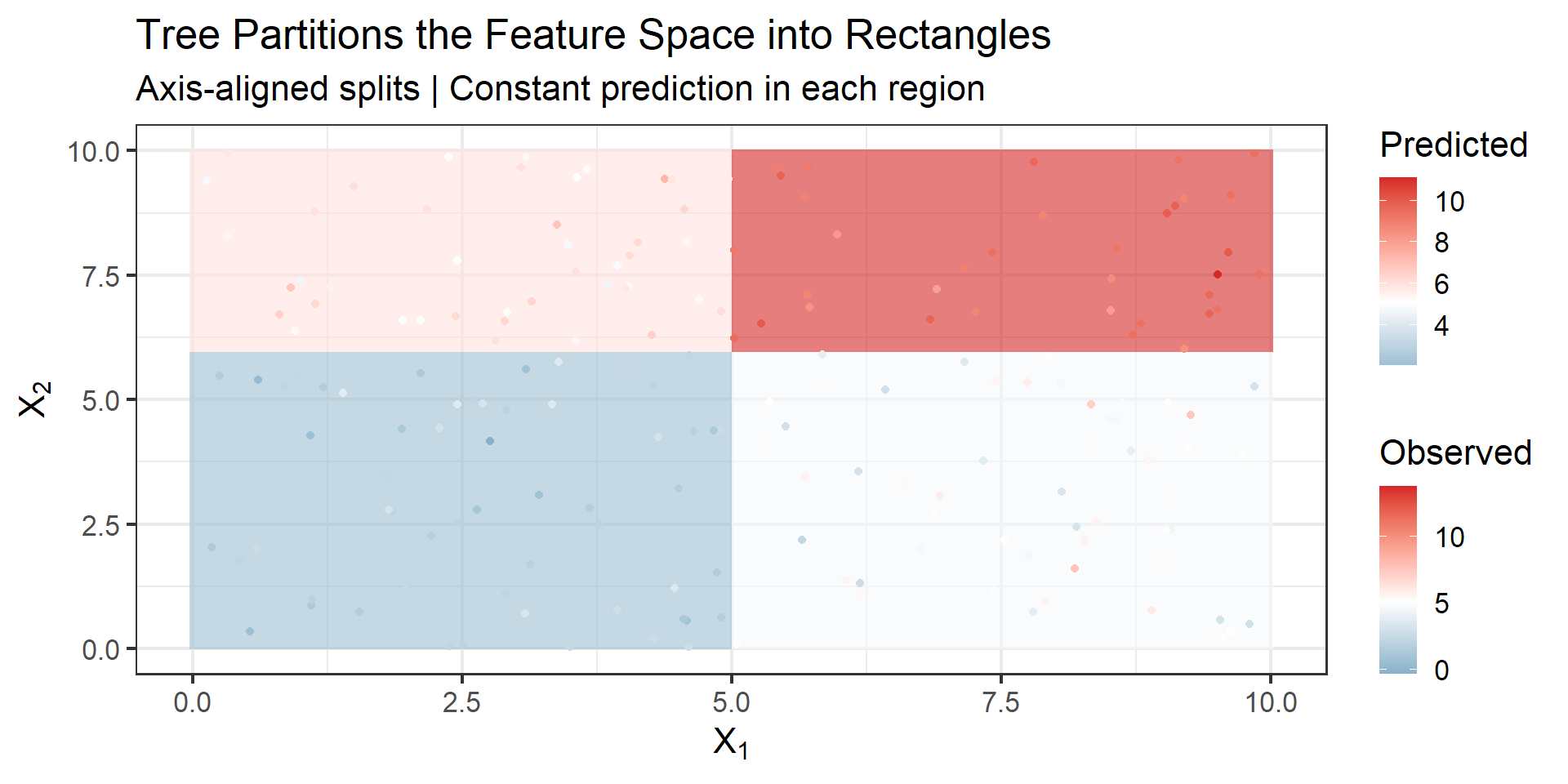
1. Partition the feature space into rectangular regions \(R_1, R_2, \ldots, R_J\)
2. Predict a constant \(\hat{c}_j\) in each region (typically the mean of \(y_i\) in \(R_j\))

\[\hat{f}(\mathbf{x}) = \sum_{j=1}^{J} \hat{c}_j \, \mathbf{1}(\mathbf{x} \in R_j)\]

No assumptions about functional form. The data decide where to split and how many regions to create.

What a Decision Tree Does

set.seed(577)
n <- 200
x1 <- runif(n, 0, 10)
x2 <- runif(n, 0, 10)
# True function: nonlinear with interactions
y <- 2 + 3 * (x1 > 5) + 4 * (x2 > 6) + 2 * (x1 > 5) * (x2 > 6) + rnorm(n, 0, 1)
tree_df <- data.frame(x1 = x1, x2 = x2, y = y)

# Fit a regression tree
tree_fit <- rpart(y ~ x1 + x2, data = tree_df,
                  control = rpart.control(maxdepth = 3, cp = 0.01))

p <- rpart.plot(tree_fit, type = 4, extra = 101, roundint = FALSE,
                box.palette = c(clr("blue"), clr("green"), clr("orange"), clr("red")),
                main = "A Simple Regression Tree",
                cex = 1.1)

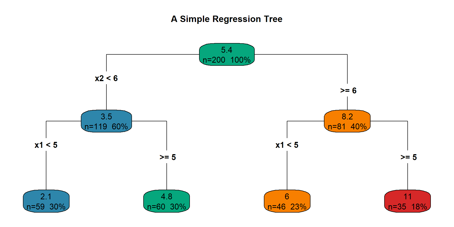
Each leaf (terminal node) contains a constant prediction: the mean of training \(y_i\) values in that region.

Reading the tree: Start at the top. At each internal node, go left if the condition is TRUE, right if FALSE.

Partition of the Feature Space

# Create grid and predict
grid <- expand.grid(x1 = seq(0, 10, length.out = 200),
                    x2 = seq(0, 10, length.out = 200))
grid$pred <- predict(tree_fit, newdata = grid)

plt <- ggplot() +
  geom_tile(data = grid, aes(x = x1, y = x2, fill = pred), alpha = 0.6) +
  geom_point(data = tree_df, aes(x = x1, y = x2, color = y), size = 1.5) +
  scale_fill_gradient2(low = clr("blue"), mid = "white", high = clr("red"),
                       midpoint = median(tree_df$y), name = "Predicted") +
  scale_color_gradient2(low = clr("blue"), mid = "white", high = clr("red"),
                        midpoint = median(tree_df$y), name = "Observed") +
  labs(title = "Tree Partitions the Feature Space into Rectangles",
       subtitle = "Axis-aligned splits | Constant prediction in each region",
       x = expression(X[1]), y = expression(X[2])) +
  theme_bw(base_size = 16)

ggsave(file.path(fig_dir, "02_tree_partition.png"), plt, width = 10, height = 5, dpi = 150)
plt

How Trees Are Built: Recursive Binary Splitting

The tree is grown top-down via a greedy algorithm.

At each step, select the predictor \(X_j\) and cutpoint \(s\) that minimize the RSS:

Splitting Criterion (Regression)

\[\min_{j,\, s} \left[\sum_{i:\, x_i \in R_1(j,s)} (y_i - \hat{c}_1)^2 + \sum_{i:\, x_i \in R_2(j,s)} (y_i - \hat{c}_2)^2\right]\]

where \(R_1(j,s) = \{\mathbf{x} \mid X_j < s\}\), \(R_2(j,s) = \{\mathbf{x} \mid X_j \ge s\}\), and \(\hat{c}_k = \text{ave}(y_i \mid \mathbf{x}_i \in R_k)\).

Greedy = best split now, no look-ahead. A seemingly poor split might enable excellent splits below it.

Continue splitting until a stopping criterion is met (e.g., minimum node size of 5).

Read: ISLR 8.1.1 for the full details of this procedure.

Classification Trees: Splitting Criteria

For classification, RSS is replaced by node impurity measures.

Let \(\hat{p}_{mk}\) = proportion of class \(k\) observations in node \(m\).

Splitting Criteria for Classification (formulas for reference)

Classification error rate: \(E = 1 - \max_k \hat{p}_{mk}\)

Gini index: \(G = \sum_{k=1}^{K} \hat{p}_{mk}(1 - \hat{p}_{mk})\)

Cross-entropy: \(D = -\sum_{k=1}^{K} \hat{p}_{mk} \log \hat{p}_{mk}\)

Week 6 connection: In Week 6 we evaluated classifiers using error rate and confusion matrices. Classification trees use node impurity measures (Gini, entropy) that are more sensitive than error rate for growing the tree.

In practice, Gini and entropy are preferred for growing the tree (more sensitive to node purity than misclassification error). For pruning, misclassification rate is often used.

Read: ISLR 8.1.2 and ESL 9.2.3 for the full classification tree algorithm.

Pruning as Regularization

A fully grown tree overfits. The solution: grow large, then prune back.

Cost-Complexity Pruning

For tuning parameter \(\alpha \ge 0\), find the subtree \(T \subseteq T_0\) that minimizes:

\[C_\alpha(T) = \sum_{m=1}^{|T|} \sum_{i:\, \mathbf{x}_i \in R_m} (y_i - \hat{y}_{R_m})^2 + \alpha |T|\]

where \(|T|\) = number of terminal nodes.

Week 3 callback: This is the same idea as regularization in linear models!

Trees	Linear Models
\(\sum \text{RSS}(R_m) + \alpha |T|\)	\(\sum (y_i - \hat{y}_i)^2 + \lambda \|\boldsymbol{\beta}\|\)
\(\alpha\) controls tree complexity	\(\lambda\) controls coefficient magnitude

\(\alpha = 0\) gives the full tree \(T_0\). As \(\alpha\) increases, the tree shrinks. Choose \(\alpha\) by cross-validation.

Read: ISLR Algorithm 8.1 for the full pruning procedure.

Trees vs Linear Models: Different Geometry

Trees vs Linear Models: Takeaway

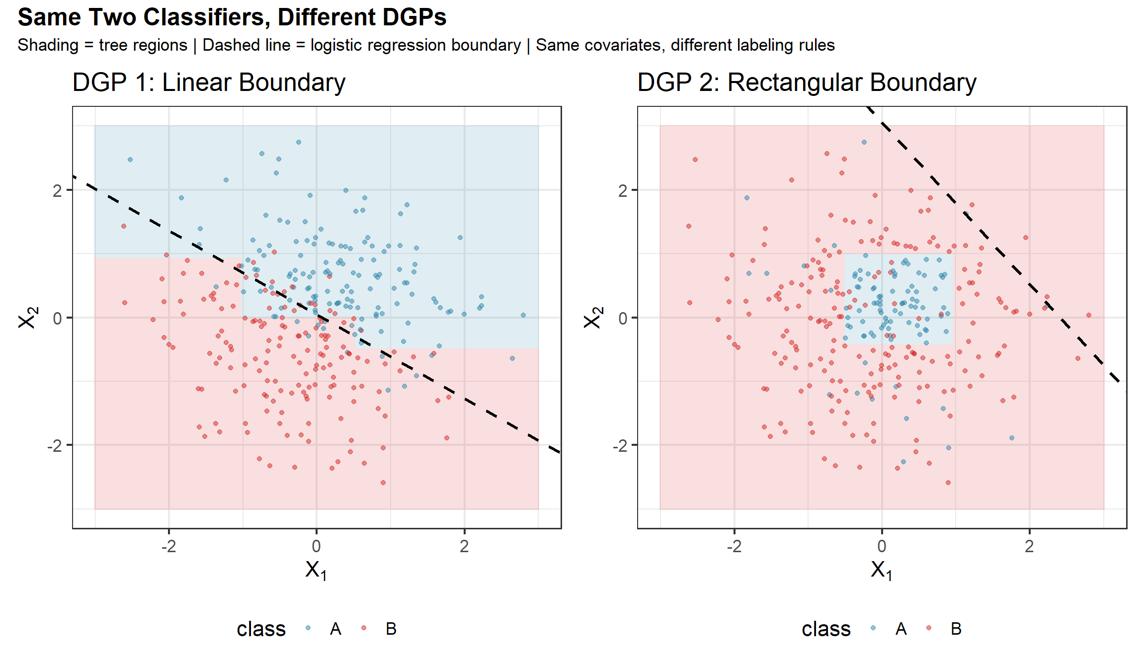
Both panels show the same two classifiers — a tree (shaded regions) and logistic regression (dashed line) — fit to data from different DGPs.

• DGP 1 (left): \(P(Y{=}A \mid \mathbf{x}) = \sigma(0.8x_1 + 1.2x_2)\) — a linear boundary.
• DGP 2 (right): \(P(Y{=}A \mid \mathbf{x}) = 0.9\) inside a rectangle, \(0.1\) outside — an axis-aligned boundary.

In practice we never know the DGP. But this illustrates why no single method dominates: the geometry of the model must match the geometry of the truth. Trees make axis-aligned splits; linear models make hyperplane cuts. Neither is universally better.

The Punchline of Block 1: Instability

set.seed(577)
n <- 150
x1 <- runif(n, 0, 10)
x2 <- runif(n, 0, 10)
y <- sin(x1) + cos(x2) + 0.5 * x1 * (x2 > 5) + rnorm(n, 0, 1)
full_df <- data.frame(x1 = x1, x2 = x2, y = y)

# Original tree
tree_orig <- rpart(y ~ x1 + x2, data = full_df,
                   control = rpart.control(maxdepth = 4, cp = 0.01))

# Bootstrap sample — different tree!
set.seed(42)
boot_idx <- sample(n, n, replace = TRUE)
boot_df <- full_df[boot_idx, ]
tree_boot <- rpart(y ~ x1 + x2, data = boot_df,
                   control = rpart.control(maxdepth = 4, cp = 0.01))

Instability: The Setup for Everything That Follows

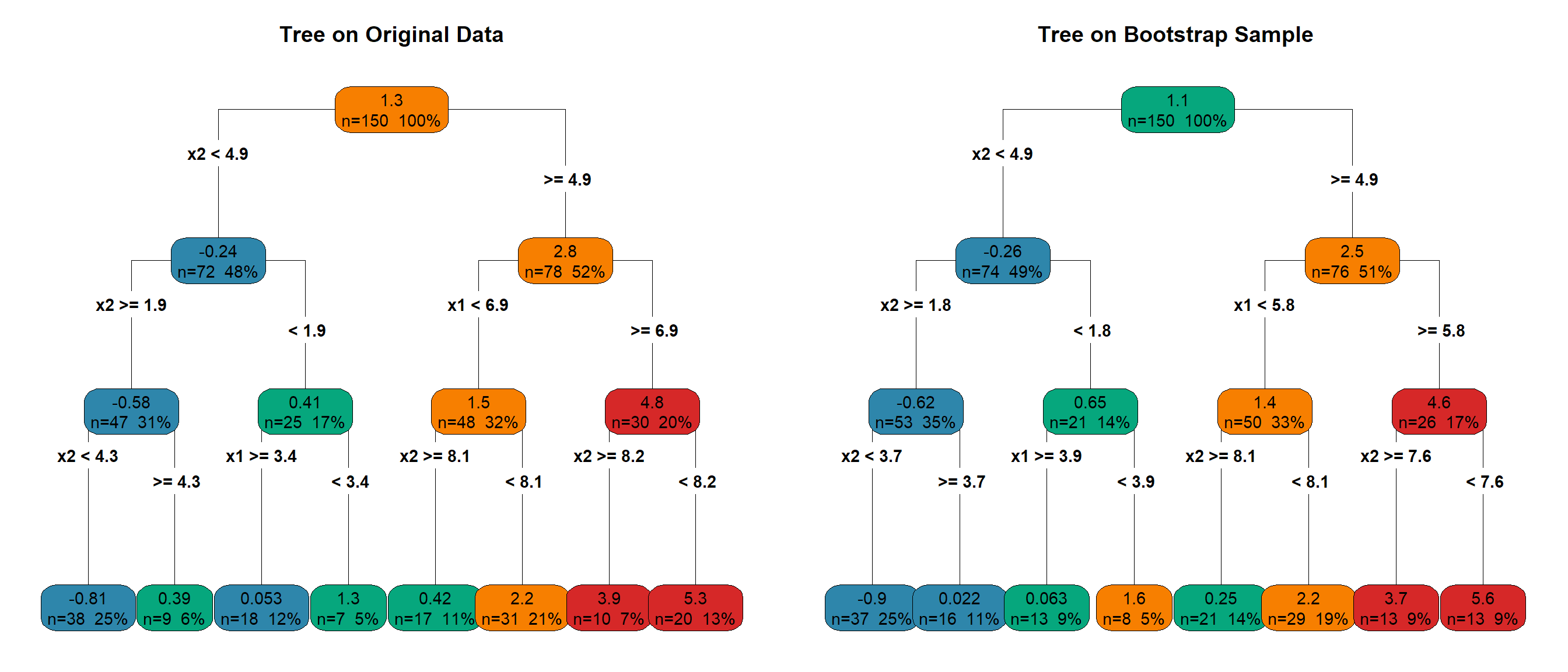
The two trees on the previous slide came from the same generating process — one is the original data, the other a bootstrap sample.

Yet the tree structures differ in important ways:

• Different cutpoints at secondary and deeper splits
• Different branching structure below the root
• Different leaf predictions (even when the root split is similar)

Trees Are High Variance, Low Bias

A deep tree can fit complex patterns (low bias), but small perturbations to the data produce very different trees (high variance).

Week 1 callback: The bias-variance tradeoff governs everything. Trees sit firmly in the high-variance corner.

The Key Insight

This instability is not a bug — it is exactly the property that makes ensembles work. If trees were stable, averaging them would not help. The rest of this deck exploits this instability.

Block 2: Bagging — Variance Reduction via Bootstrap

Week 4 Callback: Bootstrap Returns

In Week 4, we used bootstrap resampling for standard errors and confidence intervals.

The bootstrap idea: When we cannot repeatedly sample from the population, we repeatedly sample (with replacement) from the data.

Now we use bootstrap for an entirely different purpose: building better predictors.

From Week 4 to Week 7

Week 4: Bootstrap \(\to\) uncertainty quantification (SEs, CIs)

Weeks 7–8: Bootstrap \(\to\) variance reduction via averaging

Key fact from Week 4: Each bootstrap sample of size \(n\) drawn with replacement uses approximately \(1 - (1 - 1/n)^n \approx 1 - e^{-1} \approx 63.2\%\) of the unique observations.

We proved this. Now it does real work for us.

The Averaging Principle

Suppose we have \(B\) independent random variables \(Z_1, Z_2, \ldots, Z_B\), each with mean \(\mu\) and variance \(\sigma^2\).

The variance of their average is:

\[\text{Var}(\bar{Z}) = \frac{\sigma^2}{B}\]

The dream: Take \(B\) independent training sets from the population, fit a tree to each, average the predictions \(\to\) variance shrinks by factor \(B\).

The reality: We have one training set.

The fix: Use bootstrap samples as proxies for independent training sets.

The Bagging Algorithm

Bootstrap Aggregation (Bagging) — Breiman (1996)

Input: Training data \(\{(\mathbf{x}_i, y_i)\}_{i=1}^n\), number of trees \(B\)

For \(b = 1, 2, \ldots, B\):

1. Draw a bootstrap sample \(\mathcal{D}^{*b}\) of size \(n\) (with replacement) from the training data
2. Fit a deep, unpruned tree \(\hat{T}_b\) to \(\mathcal{D}^{*b}\)

Predict:

• Regression: \(\hat{f}_{\text{bag}}(\mathbf{x}) = \frac{1}{B}\sum_{b=1}^{B} \hat{T}_b(\mathbf{x})\)
• Classification: majority vote of \(\hat{T}_1(\mathbf{x}), \ldots, \hat{T}_B(\mathbf{x})\)

Critical design choice: Each tree is grown deep (no pruning). Individual trees have high variance and low bias. The averaging reduces variance without increasing bias.

But wait… bootstrap trees are not independent. They all come from the same training set. How much does averaging actually help?

Variance of Correlated Averages

This is where the math gets interesting. Let \(T_1, T_2, \ldots, T_B\) be the \(B\) trees (evaluated at a fixed \(\mathbf{x}\)).

Suppose each tree has variance \(\sigma^2\) and any pair has correlation \(\rho\).

\[\text{Var}\!\left(\frac{1}{B}\sum_{b=1}^{B} T_b\right) = \frac{1}{B^2}\left[\sum_{b=1}^{B} \text{Var}(T_b) + \sum_{b \ne b'} \text{Cov}(T_b, T_{b'})\right]\]

\[= \frac{1}{B^2}\left[B\sigma^2 + B(B-1)\rho\sigma^2\right]\]

\[= \rho\sigma^2 + \frac{1 - \rho}{B}\sigma^2\]

The Variance of an Averaged Ensemble

\[\text{Var}\!\left(\frac{1}{B}\sum_{b=1}^{B} T_b\right) = \underbrace{\rho\sigma^2}_{\text{irreducible: depends on }\rho} + \underbrace{\frac{1 - \rho}{B}\sigma^2}_{\text{vanishes as } B \to \infty}\]

Bagging drives \(B\) large, which kills the second term. But the first term — \(\rho\sigma^2\) — remains. We will return to this.

Out-of-Bag Error Estimation

Since each bootstrap sample uses only \(\approx 63.2\%\) of observations, the remaining \(\approx 36.8\%\) are “out of bag” (OOB) for each tree.

OOB prediction for observation \(i\): Average the predictions of only those trees for which observation \(i\) was not in the bootstrap sample.

\[\hat{f}_{\text{OOB}}(\mathbf{x}_i) = \frac{1}{|\mathcal{B}_i|}\sum_{b \in \mathcal{B}_i} \hat{T}_b(\mathbf{x}_i)\]

where \(\mathcal{B}_i = \{b : \text{observation } i \text{ was OOB for tree } b\}\).

Compute the OOB error by averaging \(L(y_i, \hat{f}_{\text{OOB}}(\mathbf{x}_i))\) over all \(i\).

OOB Error is (Nearly) Free Cross-Validation

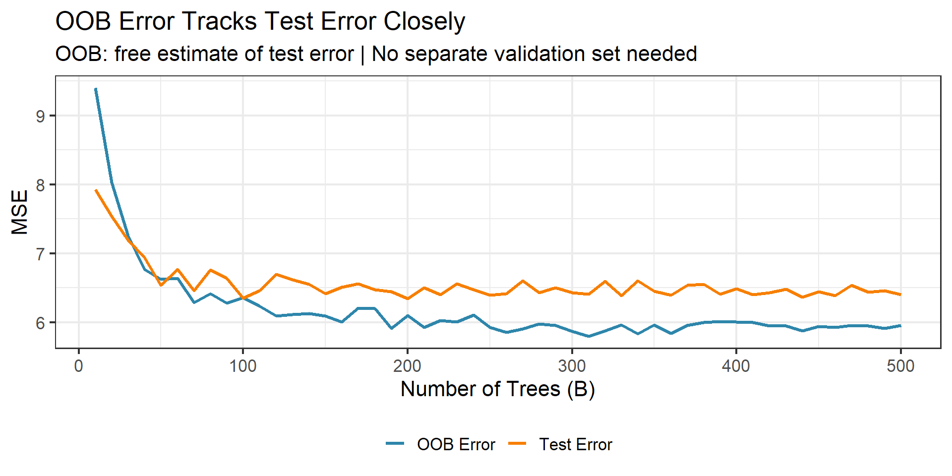
Each observation is predicted by about \(B/3\) trees that never saw it during training. As \(B \to \infty\), OOB error provides a nearly unbiased estimate of the test error — similar in spirit to cross-validation, with no additional computation.

Week 4 callback: We proved the 63.2% result. Now it works for us: each tree has a built-in test set.

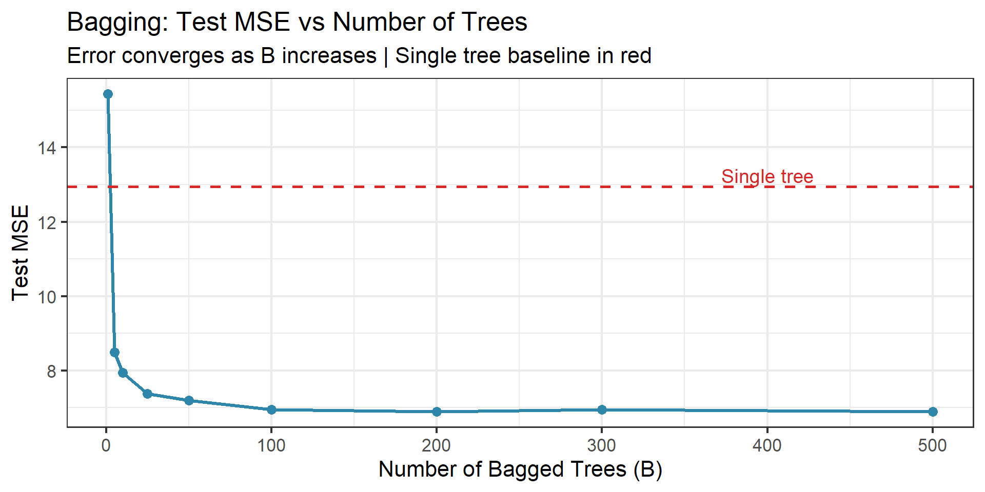
Bagging in Action: Test Error vs Number of Trees

set.seed(577)
n <- 800
p <- 20
X <- matrix(rnorm(n * p), n, p)
# X2-X10 correlated with X1 (rho ~ 0.7): creates high tree correlation for bagging
for (j in 2:10) X[, j] <- 0.7 * X[, 1] + sqrt(1 - 0.7^2) * X[, j]
colnames(X) <- paste0("X", 1:p)
# Signal distributed across correlated block + mild nonlinear term | noise sd = 2
y <- 3 * X[,1] + 2.5 * X[,2] + 2 * X[,3] + 1.5 * X[,4] + X[,5] + 0.5 * X[,11]^2 + rnorm(n, 0, 2)

train_idx <- 1:500
test_idx <- 501:800
train_df <- data.frame(y = y[train_idx], X[train_idx, ])
test_df <- data.frame(y = y[test_idx], X[test_idx, ])

# Bagging: fit randomForest with mtry = p (all predictors at each split = bagging)
B_vals <- c(1, 5, 10, 25, 50, 100, 200, 300, 500)
bag_test_errors <- sapply(B_vals, function(B) {
  set.seed(577)
  rf <- randomForest(y ~ ., data = train_df, ntree = B, mtry = p)
  pred <- predict(rf, newdata = test_df)
  mean((test_df$y - pred)^2)
})

# Single tree baseline
single_tree <- rpart(y ~ ., data = train_df, control = rpart.control(cp = 0.01))
single_pred <- predict(single_tree, newdata = test_df)
single_mse <- mean((test_df$y - single_pred)^2)

bag_df <- tibble(B = B_vals, MSE = bag_test_errors)

plt <- ggplot(bag_df, aes(x = B, y = MSE)) +
  geom_line(linewidth = 1.2, color = clr("blue")) +
  geom_point(size = 3, color = clr("blue")) +
  geom_hline(yintercept = single_mse, linetype = "dashed", color = clr("red"), linewidth = 1) +
  annotate("text", x = 400, y = single_mse + 0.3, label = "Single tree",
           color = clr("red"), size = 5) +
  labs(title = "Bagging: Test MSE vs Number of Trees",
       subtitle = "Error converges as B increases | Single tree baseline in red",
       x = "Number of Bagged Trees (B)", y = "Test MSE") +
  theme_bw(base_size = 16)

ggsave(file.path(fig_dir, "05_bagging_convergence.png"), plt, width = 10, height = 5, dpi = 150)
plt

Bagging: Summary

Bagging reduces variance by averaging many high-variance, low-bias trees.

Strengths:

• Dramatic variance reduction over single trees
• OOB error provides free test-set estimates
• \(B\) is not a critical parameter — cannot overfit by increasing \(B\)

Limitation:

\[\text{Var}(\bar{T}) = \rho\sigma^2 + \frac{1-\rho}{B}\sigma^2\]

Even with \(B = \infty\), we are left with \(\rho\sigma^2\). If one predictor dominates, all trees split on it first \(\to\) trees are correlated \(\to\) \(\rho\) is large \(\to\) averaging helps less than we would like.

Can we reduce \(\rho\)?

Block 3: Random Forests — The Decorrelation Trick

The Centerpiece of Weeks 7–8

Random forests attack the correlation between trees. This is where the magic happens.

The Problem with Bagging

Consider a dataset where one predictor \(X_1\) is much stronger than the rest.

Every bagged tree will split on \(X_1\) first. The trees look similar in structure:

Tree 1: X1 < 5.2 → ...     Tree 2: X1 < 5.1 → ...     Tree 3: X1 < 5.3 → ...

The trees are highly correlated. The pairwise correlation \(\rho\) is close to 1.

From our variance formula:

\[\text{Var}(\bar{T}) = \rho\sigma^2 + \frac{1 - \rho}{B}\sigma^2 \approx \sigma^2 \quad \text{when } \rho \approx 1\]

Averaging many nearly identical trees barely reduces variance. We need diversity.

Breiman’s Fix: Random Feature Selection

Random Forests — Breiman (2001)

At each split in each tree, randomly select \(m\) out of \(p\) predictors as candidates.

Only these \(m\) predictors may be considered for the split.

A fresh random subset is drawn at every split.

When \(m = p\): this is just bagging (all predictors available).

When \(m = 1\): splits are completely random (too aggressive).

Rules of thumb:

• Classification: \(m \approx \sqrt{p}\)
• Regression: \(m \approx p/3\)

By restricting the candidate set, we force the trees to be different. Even with a dominant predictor, on average \((p - m)/p\) of the splits will not even consider it.

The Key Formula: Why Random Forests Work

Recall the variance decomposition:

\[\text{Var}\!\left(\frac{1}{B}\sum_{b=1}^{B} T_b\right) = \rho\sigma^2 + \frac{1-\rho}{B}\sigma^2\]

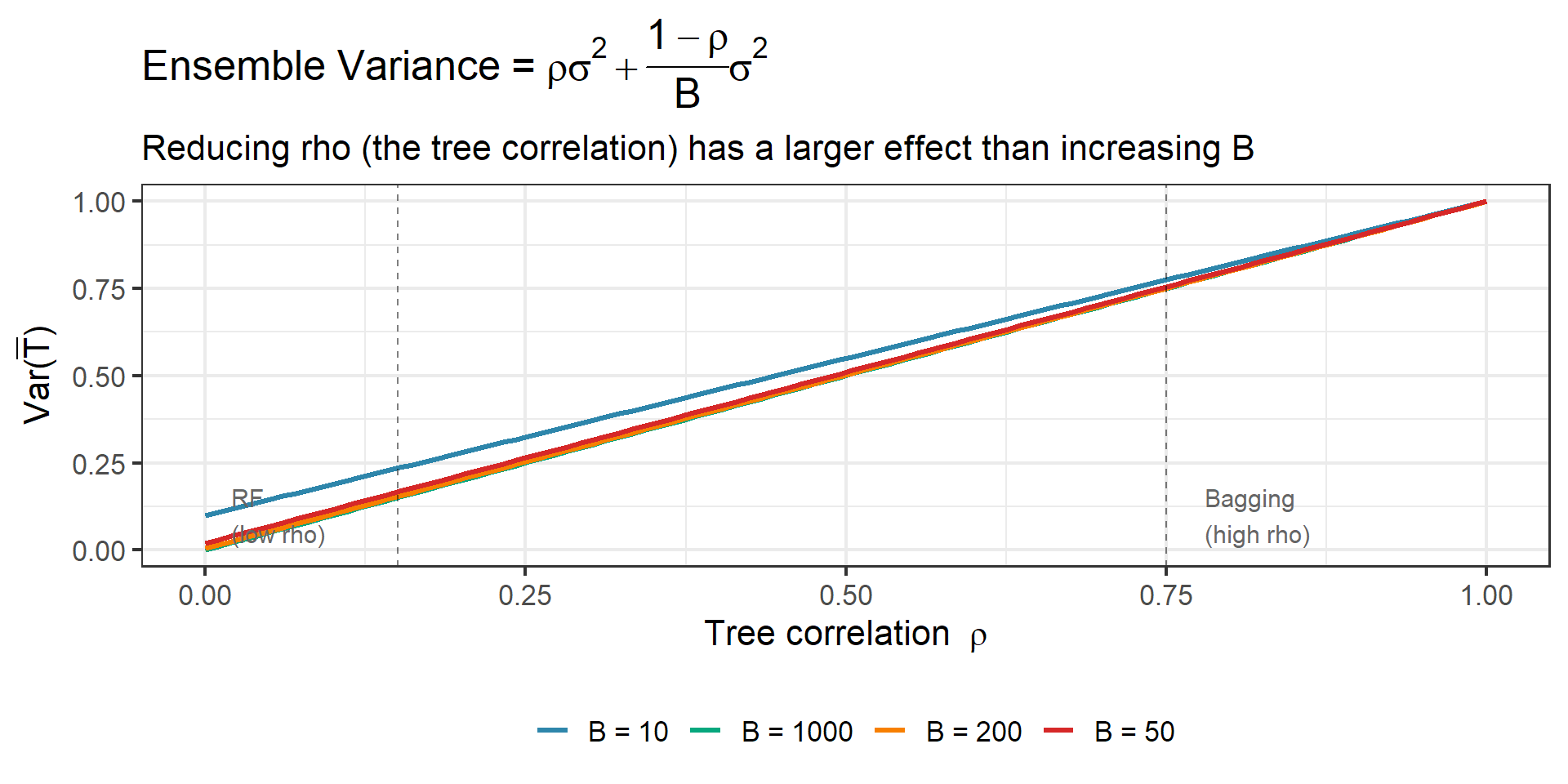
Bagging (\(m = p\)): Increases \(B\) \(\to\) kills the second term. But \(\rho\) is large because all trees see the same strong predictors. First term dominates.

Random forests (\(m < p\)): Also increases \(B\), and reduces \(\rho\) by decorrelating the trees.

The Decorrelation Argument

\[\underbrace{\text{Var}(\bar{T})}_{\text{ensemble variance}} = \underbrace{\rho\sigma^2}_{\substack{\text{RF attacks this} \\ \text{by reducing } \rho}} + \underbrace{\frac{1-\rho}{B}\sigma^2}_{\substack{\text{both RF and bagging} \\ \text{attack this via } B \to \infty}}\]

Bagging attacks only the second term.

Random forests attack both terms.

This is the fundamental reason RF outperforms bagging.

Deriving the Variance Formula

Let us derive this carefully. For a fixed test point \(\mathbf{x}\), let \(T_b = T_b(\mathbf{x})\) be the prediction of tree \(b\).

Assumptions:

• Each \(T_b\) has mean \(\mu\) and variance \(\sigma^2\)
• Each pair \((T_b, T_{b'})\) has correlation \(\rho\) (the average pairwise correlation)

Then: \[\text{Var}\!\left(\frac{1}{B}\sum_{b=1}^{B} T_b\right) = \frac{1}{B^2} \text{Var}\!\left(\sum_{b=1}^{B} T_b\right)\]

\[= \frac{1}{B^2}\left[\sum_{b=1}^{B}\sigma^2 + \sum_{b \ne b'} \rho\sigma^2\right] = \frac{1}{B^2}\left[B\sigma^2 + B(B-1)\rho\sigma^2\right]\]

\[= \frac{\sigma^2}{B} + \frac{B-1}{B}\rho\sigma^2 = \frac{\sigma^2}{B}(1 - \rho) + \rho\sigma^2\]

As \(B \to \infty\): \(\text{Var}(\bar{T}) \to \rho\sigma^2\). The floor is set by the correlation between trees.

Visualizing the Decorrelation

The RF Algorithm

Random Forest Algorithm

Input: Training data, number of trees \(B\), candidate features per split \(m\)

For \(b = 1, 2, \ldots, B\):

1. Draw a bootstrap sample \(\mathcal{D}^{*b}\) from the training data
2. Grow a tree \(\hat{T}_b\) on \(\mathcal{D}^{*b}\):
   • At each node, select \(m\) features at random from all \(p\) features
   • Among these \(m\), find the best split (by RSS or Gini/entropy)
   • Split the node; continue until minimum node size is reached
   • Do not prune

Predict: Average (regression) or majority vote (classification)

Two sources of randomness:

1. Bootstrap sampling of observations (inherited from bagging)
2. Random feature selection at each split (new in RF)

Both contribute to decorrelation.

Random Forest: Code Demo

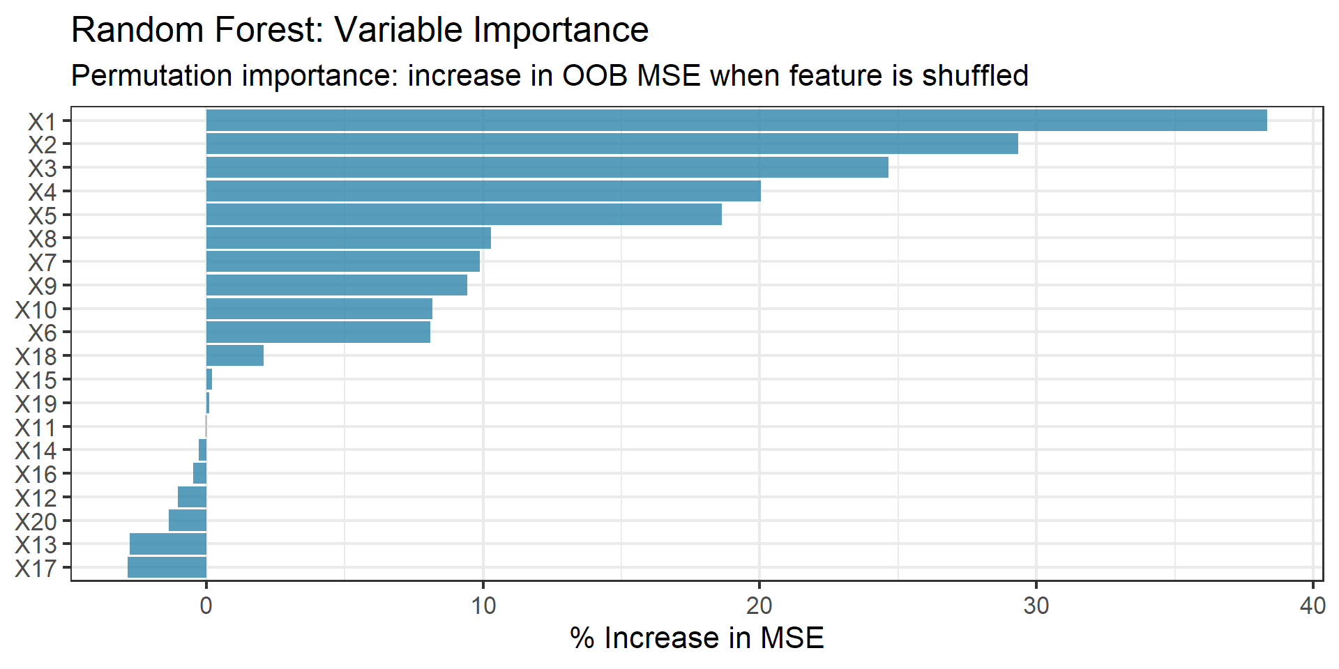
set.seed(577)
# Using the same simulated data from bagging demo
rf_fit <- randomForest(y ~ ., data = train_df, ntree = 500,
                       mtry = floor(p / 3),  # p/3 for regression
                       importance = TRUE)

# Variable importance plot
imp_df <- tibble(
  Variable = rownames(importance(rf_fit)),
  IncMSE = importance(rf_fit)[, "%IncMSE"]
) |> arrange(desc(IncMSE))

plt <- ggplot(imp_df, aes(x = reorder(Variable, IncMSE), y = IncMSE)) +
  geom_col(fill = clr("blue"), alpha = 0.8) +
  coord_flip() +
  labs(title = "Random Forest: Variable Importance",
       subtitle = "Permutation importance: increase in OOB MSE when feature is shuffled",
       x = NULL, y = "% Increase in MSE") +
  theme_bw(base_size = 16)

ggsave(file.path(fig_dir, "07_rf_variable_importance.png"), plt, width = 10, height = 5, dpi = 150)
plt

Variable Importance: How It Works

Permutation importance for variable \(X_j\):

1. Compute OOB error for each tree (using unpermuted data)
2. Randomly permute the values of \(X_j\) in the OOB data
3. Re-compute OOB error with \(X_j\) permuted
4. Importance = average increase in error across all trees

If \(X_j\) is important, permuting it destroys its predictive signal \(\to\) large increase in error.

Limitations of Permutation Importance

• Correlated features: If \(X_j\) and \(X_k\) are correlated, permuting \(X_j\) creates unrealistic \((X_j, X_k)\) combinations. Importance may be split between correlated features or underestimated.
• Cardinality bias: Features with more distinct values get more split opportunities in individual trees.

See Strobl et al. (2007) for a careful analysis. Conditional permutation importance addresses some of these issues, but at higher computational cost.

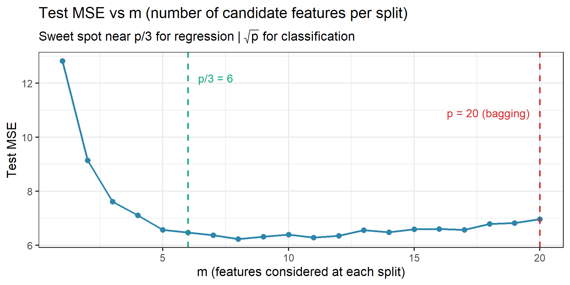
Choosing \(m\): The Tuning Sweet Spot

OOB Error vs Test Error

Week 4 Callback: OOB = Free CV

The 63.2% bootstrap inclusion result from Week 4 gives us a free test-set estimate. As \(B \to \infty\), each observation’s OOB prediction stabilizes, providing a nearly unbiased estimate of test error.

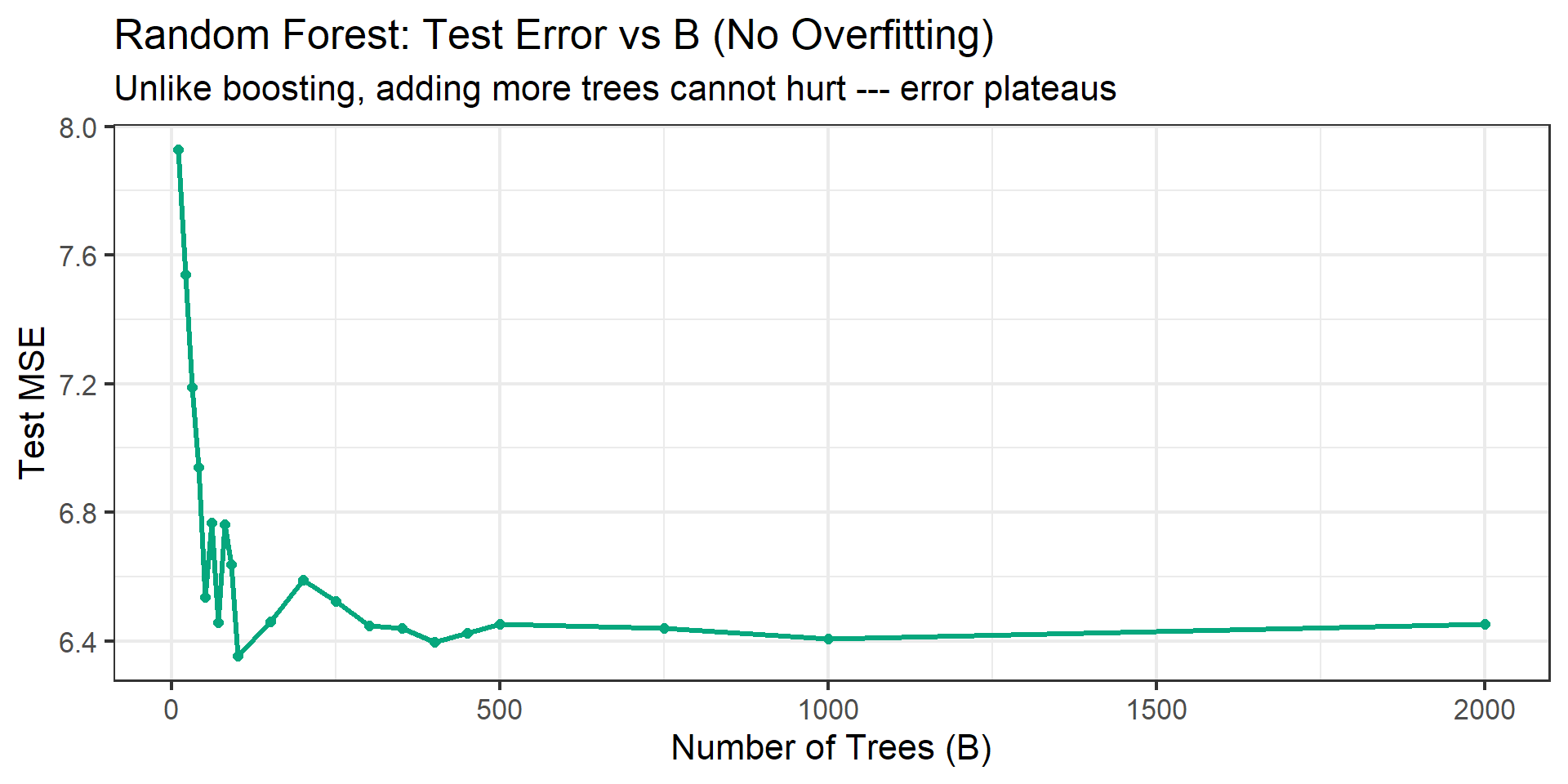
RF Does Not Overfit as \(B\) Increases

Key Property

Random forests cannot overfit by increasing \(B\). Each additional tree is fit to a new bootstrap sample and averaged in. The variance formula \(\rho\sigma^2 + \frac{1-\rho}{B}\sigma^2\) only decreases (or stays flat) as \(B\) grows. This is a major practical advantage.

Breiman (2001): Key Insights

1. Upper bound on generalization error:

Breiman shows that the generalization error of a random forest is bounded by:

\[PE^* \le \frac{\bar{\rho}(1 - s^2)}{s^2}\]

where \(\bar{\rho}\) is the mean correlation between trees and \(s\) measures the “strength” of individual trees (their expected margin).

2. The strength-correlation tradeoff:

• Decreasing \(m\) \(\to\) decreases correlation \(\bar{\rho}\) (good!) but also decreases strength \(s\) (bad!)
• The optimal \(m\) balances these two forces
• Rules of thumb \(\sqrt{p}\) and \(p/3\) work because they approximately optimize this tradeoff

3. Consistency:

Under regularity conditions, random forests are consistent: as \(n \to \infty\) and the forest grows, predictions converge to the true regression function. Formal proofs require careful treatment of the adaptive splitting; see Biau & Scornet (2016) for modern results.

4. Why “random” is the point:

The randomness is not a nuisance — it is the mechanism that creates diversity. Without it, we have correlated bagged trees and limited variance reduction.

Breiman’s Bound: Intuition

Breiman’s Generalization Bound (2001)

\[PE^* \le \frac{\bar{\rho}(1 - s^2)}{s^2}\]

• \(s\) = strength: expected margin of a single tree (\(s\) large \(\to\) each tree is accurate)
• \(\bar{\rho}\) = mean correlation: how similar the trees are (\(\bar{\rho}\) small \(\to\) trees are diverse)

Reading the bound:

• Numerator: \(\bar{\rho}(1 - s^2)\) — high correlation and imperfect individual trees drive error up
• Denominator: \(s^2\) — stronger individual trees reduce the bound
• \(\bar{\rho}/s^2\) is the critical ratio — we want low correlation relative to high strength

This formalizes the intuition: The best ensemble has strong but diverse members.

This is not unique to trees — the same principle governs any ensemble method. But random feature selection gives us a direct knob to turn.

Block 4: Boosting — Sequential Error Correction

A Different Philosophy

Bagging / RF: Fit trees independently (in parallel), then average.

Boosting: Fit trees sequentially, each correcting the errors of the ensemble so far.

Bagging / RF

• Trees are independent
• Each tree is deep (low bias, high variance)
• Averaging reduces variance
• Cannot overfit with more trees

Boosting

• Trees are sequential and dependent
• Each tree is shallow (high bias, low variance)
• Sequential correction reduces bias
• Can overfit with too many trees

AdaBoost: A Brief Sketch

AdaBoost (Freund & Schapire, 1997) was the original boosting algorithm for classification.

AdaBoost.M1 — Sketch

1. Initialize weights \(w_i = 1/n\) for all observations
2. For \(m = 1, 2, \ldots, M\):
   • Fit a classifier \(G_m(\mathbf{x})\) using weights \(w_i\)
   • Compute weighted error: \(\text{err}_m = \sum_i w_i \, \mathbf{1}(y_i \ne G_m(\mathbf{x}_i)) \Big/ \sum_i w_i\)
   • Compute classifier weight: \(\alpha_m = \log\!\left(\frac{1 - \text{err}_m}{\text{err}_m}\right)\)
   • Update: \(w_i \leftarrow w_i \cdot \exp[\alpha_m \, \mathbf{1}(y_i \ne G_m(\mathbf{x}_i))]\)
3. Output: \(G(\mathbf{x}) = \text{sign}\!\left(\sum_{m=1}^{M} \alpha_m G_m(\mathbf{x})\right)\)

Key idea: Misclassified observations get higher weights \(\to\) the next classifier focuses on the hard cases.

Friedman, Hastie & Tibshirani (2000) showed that AdaBoost is equivalent to forward stagewise additive modeling with exponential loss. We will not derive this — the gradient boosting framework below is more general and more illuminating.

Gradient Boosting for Regression

The workhorse of modern boosting. Start simple, build up slowly.

Gradient Boosting Algorithm (Regression)

1. Initialize: \(\hat{f}^{(0)}(\mathbf{x}) = \bar{y}\) (predict the mean)
2. For \(b = 1, 2, \ldots, B\):
   • Compute residuals: \(r_i = y_i - \hat{f}^{(b-1)}(\mathbf{x}_i)\)
   • Fit a shallow tree \(\hat{h}_b\) (with \(d\) splits) to the residuals \((r_i, \mathbf{x}_i)\)
   • Update: \(\hat{f}^{(b)}(\mathbf{x}) = \hat{f}^{(b-1)}(\mathbf{x}) + \lambda \, \hat{h}_b(\mathbf{x})\)
3. Output: \(\hat{f}(\mathbf{x}) = \bar{y} + \sum_{b=1}^{B} \lambda \, \hat{h}_b(\mathbf{x})\)

Each tree is fit to the current residuals — the signal that the ensemble has not yet captured.

The shrinkage parameter \(\lambda \in (0, 1)\) slows down the learning. Typical values: \(\lambda = 0.01\) or \(0.001\).

Why Residuals? Gradient Descent in Function Space

Here is the conceptual leap. For squared error loss \(L(y, f) = \frac{1}{2}(y - f)^2\):

The negative gradient of the loss with respect to \(f(\mathbf{x}_i)\) is:

\[-\frac{\partial L(y_i, f(\mathbf{x}_i))}{\partial f(\mathbf{x}_i)} = y_i - f(\mathbf{x}_i) = r_i\]

The residuals are the negative gradient of the squared error loss!

Gradient Boosting = Gradient Descent in Function Space

At each step, we move the function \(\hat{f}\) in the direction that most reduces the loss. For squared error, that direction is “toward the residuals.” But the idea generalizes:

• Absolute error loss: negative gradient = \(\text{sign}(r_i)\)
• Huber loss: compromise between squared and absolute
• Cross-entropy loss (classification): negative gradient = \(y_i - p_i\) (observed minus predicted probability)

Gradient boosting = fit trees to the negative gradient of any differentiable loss function.

The General Gradient Boosting Framework

Gradient Tree Boosting — General Form (after ESL Ch. 10)

1. Initialize \(f_0(\mathbf{x}) = \arg\min_\gamma \sum_{i=1}^{n} L(y_i, \gamma)\)
2. For \(m = 1, 2, \ldots, M\):
   • Compute pseudo-residuals: \(r_{im} = -\left[\frac{\partial L(y_i, f(\mathbf{x}_i))}{\partial f(\mathbf{x}_i)}\right]_{f = f_{m-1}}\)
   • Fit a regression tree to targets \(r_{im}\), producing terminal regions \(R_{jm}\)
   • For each region, compute optimal constant: \(\gamma_{jm} = \arg\min_\gamma \sum_{\mathbf{x}_i \in R_{jm}} L(y_i, f_{m-1}(\mathbf{x}_i) + \gamma)\)
   • Update: \(f_m(\mathbf{x}) = f_{m-1}(\mathbf{x}) + \lambda \sum_j \gamma_{jm} \, \mathbf{1}(\mathbf{x} \in R_{jm})\)
3. Output \(\hat{f}(\mathbf{x}) = f_M(\mathbf{x})\)

Loss function	Negative gradient (pseudo-residual)	Setting
\(\frac{1}{2}(y - f)^2\)	\(y_i - f(\mathbf{x}_i)\)	Regression
\(|y - f|\)	\(\text{sign}(y_i - f(\mathbf{x}_i))\)	Robust regression
Multinomial deviance	\(I(y_i = k) - p_k(\mathbf{x}_i)\)	Classification

The unified framework: whatever the loss, compute the gradient, fit a tree to it, take a step.

The Three Tuning Parameters of Boosting

Boosting Has Three Knobs to Tune

1. Number of trees \(B\)

• Unlike RF, boosting can overfit if \(B\) is too large
• Use cross-validation or early stopping to select \(B\)

2. Shrinkage rate \(\lambda\) (learning rate)

• Controls how much each tree contributes
• Small \(\lambda\) (0.001–0.01) \(\to\) needs large \(B\), but generally performs better
• “Slow learning” is the key principle

3. Interaction depth \(d\) (number of splits per tree)

• \(d = 1\): stumps \(\to\) additive model (no interactions)
• \(d = 2\): allows pairwise interactions
• \(d = 3\)–\(8\): typical range in practice
• Higher \(d\) = more complex individual trees

Week 3 callback: The shrinkage \(\lambda\) in boosting is regularization — the same concept as \(\lambda\|\boldsymbol{\beta}\|\) in ridge/lasso, and \(\alpha|T|\) in tree pruning.

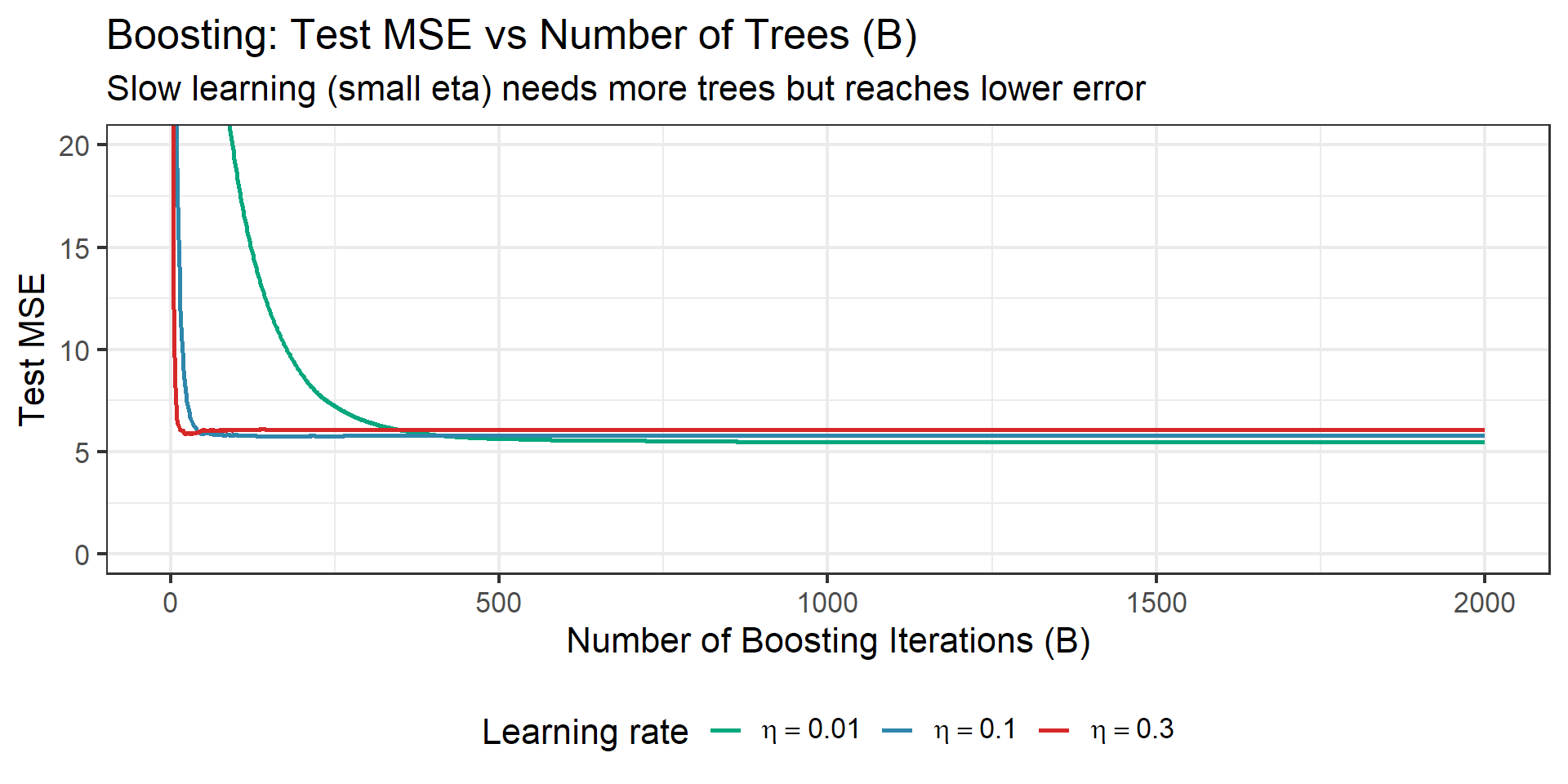
Boosting: Slow Learning Wins

set.seed(577)
# Prepare data for xgboost
dtrain <- xgb.DMatrix(data = as.matrix(train_df[, -1]), label = train_df$y)
dtest <- xgb.DMatrix(data = as.matrix(test_df[, -1]), label = test_df$y)

# Fit with different learning rates and track test error
# Tested with xgboost 3.2.0.1 — callback API changed in 3.x (evals, not watchlist)
results <- list()
for (eta_val in c(0.3, 0.1, 0.01)) {
  cb <- xgb.cb.evaluation.log()
  model <- xgb.train(
    params = list(objective = "reg:squarederror", eta = eta_val, max_depth = 4,
                  nthread = 1),
    data = dtrain, nrounds = 2000, verbose = 0,
    evals = list(train = dtrain, test = dtest),
    callbacks = list(cb)
  )
  log_df <- do.call(rbind, lapply(cb$env$evaluation_log, function(entry) {
    data.frame(iter = entry$iter, test_rmse = entry$metrics[["test-rmse"]])
  }))
  results[[as.character(eta_val)]] <- tibble(
    iteration = log_df$iter,
    MSE = log_df$test_rmse^2,
    eta = paste0("eta == ", eta_val)
  )
}

boost_df <- bind_rows(results)

plt <- ggplot(boost_df, aes(x = iteration, y = MSE, color = eta)) +
  geom_line(linewidth = 1) +
  scale_color_manual(values = c("eta == 0.3" = clr("red"), "eta == 0.1" = clr("blue"),
                                "eta == 0.01" = clr("green")),
                     name = "Learning rate",
                     labels = scales::label_parse()) +
  labs(title = "Boosting: Test MSE vs Number of Trees (B)",
       subtitle = "Slow learning (small eta) needs more trees but reaches lower error",
       x = "Number of Boosting Iterations (B)", y = "Test MSE") +
  coord_cartesian(ylim = c(0, 20)) +
  theme_bw(base_size = 16) +
  theme(legend.position = "bottom")

ggsave(file.path(fig_dir, "11_boosting_learning_rate.png"), plt, width = 10, height = 5, dpi = 150)
plt

Why Doesn’t XGBoost Overfit Here?

In theory, boosting can overfit if \(B\) is too large — each additional tree may fit noise. In practice, XGBoost’s built-in regularization (\(L_2\) penalty on leaf weights, minimum loss reduction \(\gamma\)) prevents test error from increasing. The test error plateaus rather than rising.

But slow learning still wins: \(\eta = 0.01\) ultimately reaches lower error than \(\eta = 0.3\), at the cost of needing many more iterations. Early stopping selects the optimal \(B\) and saves computation.

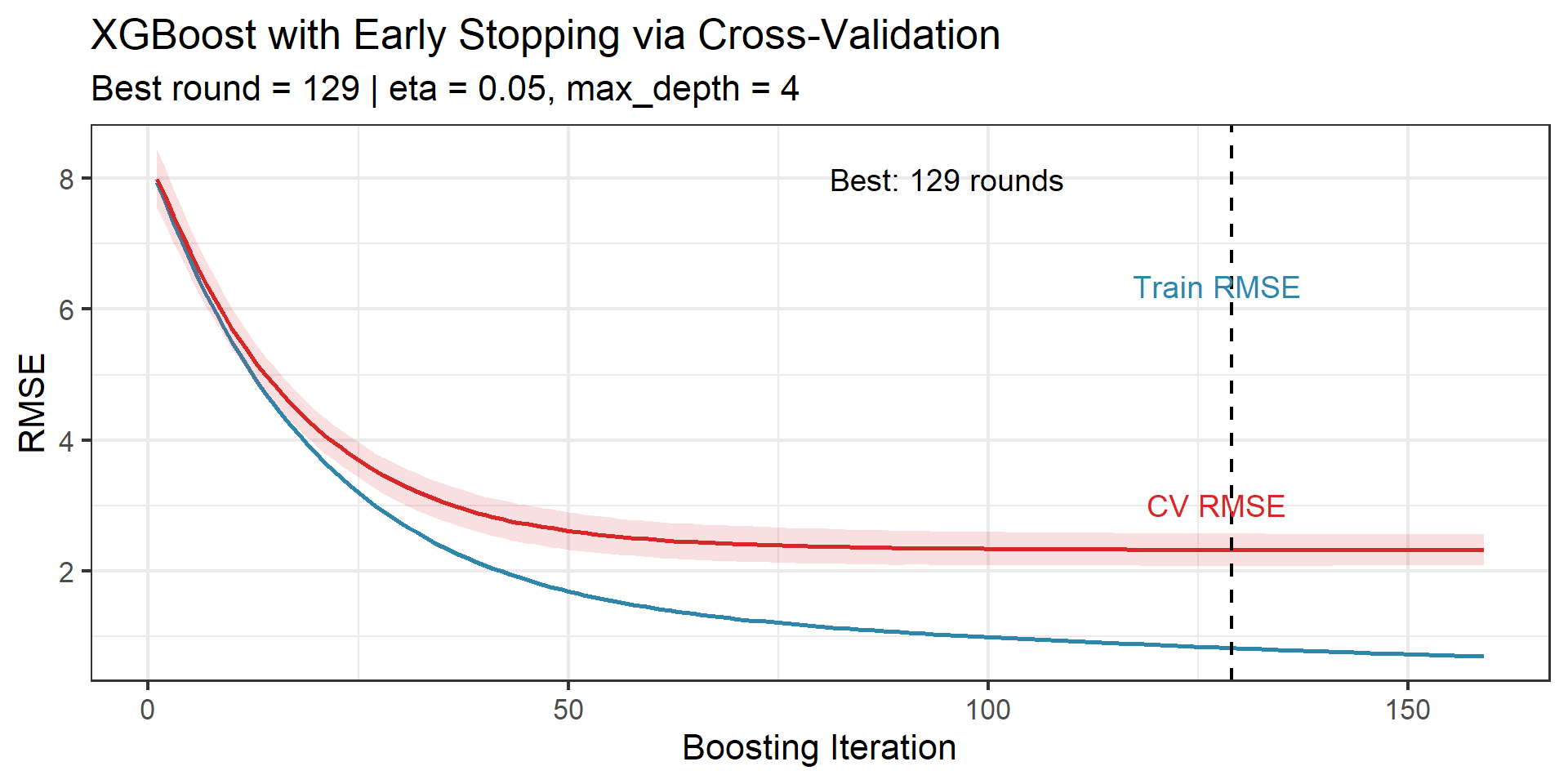
XGBoost: Gradient Boosting in Practice

set.seed(577)
# XGBoost with cross-validation for early stopping
xgb_cv <- xgb.cv(
  params = list(
    objective = "reg:squarederror",
    eta = 0.05,          # learning rate (shrinkage)
    max_depth = 4,       # interaction depth
    subsample = 0.8,     # row sampling (like bagging within boosting)
    colsample_bytree = 0.8,  # column sampling (like RF within boosting)
    nthread = 1
  ),
  data = dtrain,
  nrounds = 2000,
  nfold = 5,
  early_stopping_rounds = 30,
  verbose = 0
)

# Best iteration (xgboost 3.x: moved to early_stop)
best_round <- xgb_cv$early_stop$best_iteration

# evaluation_log is a data.table in xgb.cv (columns: iter, train_rmse_mean, etc.)
cv_log <- as.data.frame(xgb_cv$evaluation_log)

plt <- ggplot(cv_log, aes(x = iter)) +
  geom_line(aes(y = train_rmse_mean), color = clr("blue"), linewidth = 1) +
  geom_line(aes(y = test_rmse_mean), color = clr("red"), linewidth = 1) +
  geom_ribbon(aes(ymin = test_rmse_mean - test_rmse_std,
                  ymax = test_rmse_mean + test_rmse_std),
              alpha = 0.15, fill = clr("red")) +
  geom_vline(xintercept = best_round, linetype = "dashed", linewidth = 0.8) +
  annotate("text", x = best_round - 20, y = max(cv_log$test_rmse_mean),
           label = paste0("Best: ", best_round, " rounds"),
           hjust = 1, size = 5) +
  annotate("text", x = max(cv_log$iter) * 0.8, y = max(cv_log$train_rmse_mean) * 0.8,
           label = "Train RMSE", color = clr("blue"), size = 5) +
  annotate("text", x = max(cv_log$iter) * 0.8, y = min(cv_log$test_rmse_mean) * 1.3,
           label = "CV RMSE", color = clr("red"), size = 5) +
  labs(title = "XGBoost with Early Stopping via Cross-Validation",
       subtitle = paste0("Best round = ", best_round, " | eta = 0.05, max_depth = 4"),
       x = "Boosting Iteration", y = "RMSE") +
  theme_bw(base_size = 16)

ggsave(file.path(fig_dir, "12_xgboost_cv.png"), plt, width = 10, height = 5, dpi = 150)
plt

XGBoost / LightGBM: Modern Implementations

XGBoost (Chen & Guestrin, 2016) and LightGBM (Ke et al., 2017) are the dominant gradient boosting implementations.

Key innovations beyond the basic algorithm:

• Regularized objective: XGBoost adds \(L_1\) and \(L_2\) penalties on leaf weights, plus a penalty on the number of leaves — regularization built into the loss function itself
• Column sampling: Like RF, sample a random subset of features at each tree or split \(\to\) decorrelation within boosting
• Row subsampling: Use a random fraction of the training data for each tree
• Histogram-based splits: LightGBM bins continuous features into histograms for faster split finding
• GPU acceleration: Both support GPU training for large datasets
• Handling of missing values: Built-in handling without imputation

Practical Recommendation

For maximum predictive accuracy with structured/tabular data, gradient boosting (XGBoost or LightGBM) is the default first choice in applied machine learning. Random forests are the low-tuning alternative.

Boosting as Bias Reduction: The Clean Contrast

Bagging/RF vs Boosting: Complementary Strategies

	Bagging / RF	Boosting
Base learners	Deep trees (low bias, high variance)	Shallow trees (high bias, low variance)
Combination	Parallel + averaging	Sequential + additive
Primary effect	Variance reduction	Bias reduction
Mechanism	Averaging decorrelated trees reduces \(\text{Var}\)	Iterative residual-fitting reduces \(\text{Bias}^2\)
Overfitting	Cannot overfit with more trees	Can overfit with too many trees
Key tuning	\(m\) (features per split)	\(B\), \(\lambda\), \(d\)

Bias-Variance Insight

Bagging/RF: Start with complex trees (low bias, high variance) \(\to\) reduce variance by averaging

Boosting: Start with simple trees (high bias, low variance) \(\to\) reduce bias by iterative correction

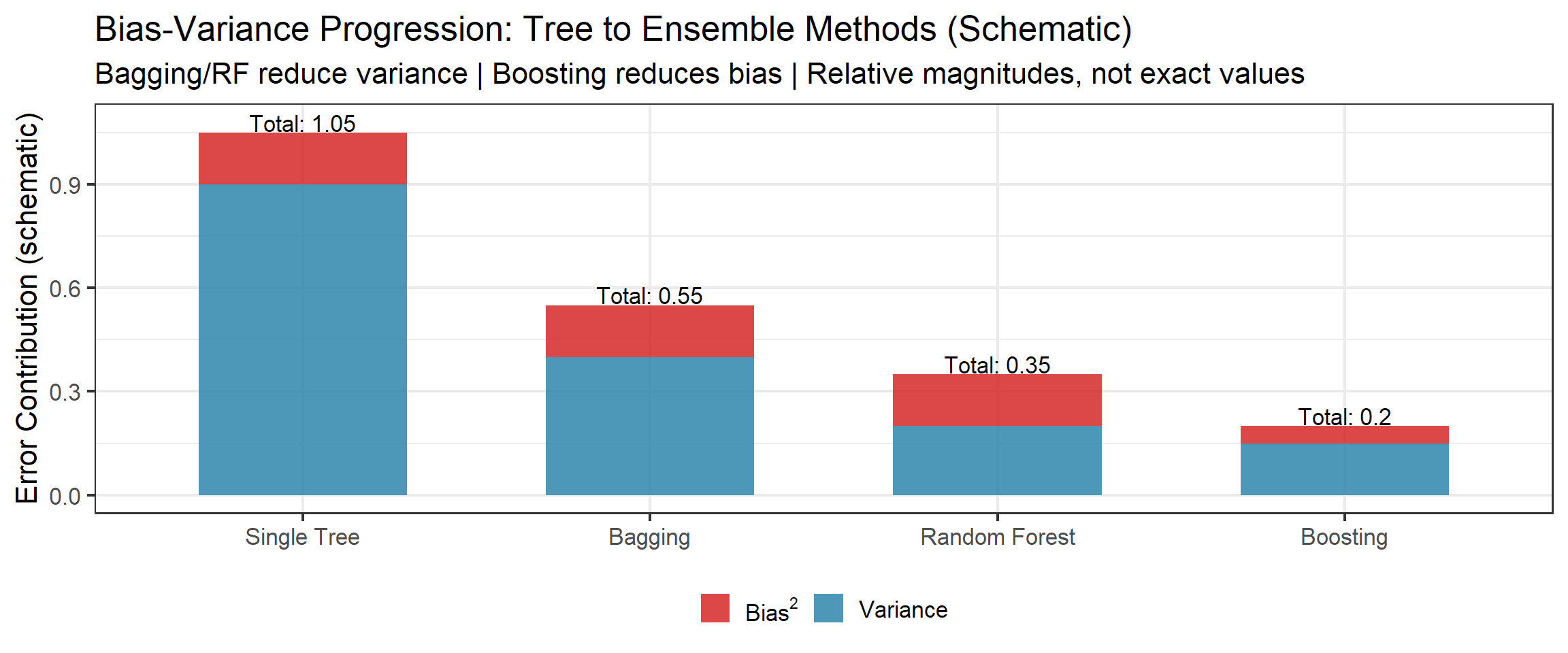
These are complementary strategies for attacking different sides of the bias-variance decomposition from Week 1.

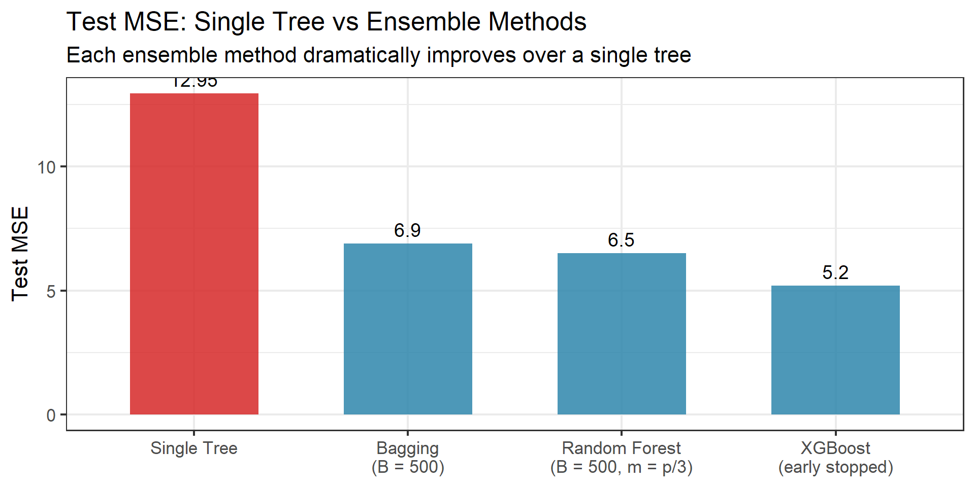
Head-to-Head Comparison

set.seed(577)

# Single tree
tree_pred <- predict(single_tree, newdata = test_df)
tree_mse <- mean((test_df$y - tree_pred)^2)

# Bagging (mtry = p)
bag_fit <- randomForest(y ~ ., data = train_df, ntree = 500, mtry = p)
bag_pred <- predict(bag_fit, newdata = test_df)
bag_mse <- mean((test_df$y - bag_pred)^2)

# Random Forest (mtry = p/3)
rf_pred <- predict(rf_fit, newdata = test_df)
rf_mse <- mean((test_df$y - rf_pred)^2)

# XGBoost
xgb_final <- xgb.train(
  params = list(objective = "reg:squarederror", eta = 0.05, max_depth = 4,
                subsample = 0.8, colsample_bytree = 0.8, nthread = 1),
  data = dtrain, nrounds = best_round, verbose = 0
)
xgb_pred <- predict(xgb_final, dtest)
xgb_mse <- mean((test_df$y - xgb_pred)^2)

comp_df <- tibble(
  Method = c("Single Tree", "Bagging\n(B = 500)", "Random Forest\n(B = 500, m = p/3)",
             "XGBoost\n(early stopped)"),
  MSE = c(tree_mse, bag_mse, rf_mse, xgb_mse),
  Type = c("Single", "Ensemble", "Ensemble", "Ensemble")
)
comp_df$Method <- factor(comp_df$Method, levels = comp_df$Method)

plt <- ggplot(comp_df, aes(x = Method, y = MSE, fill = Type)) +
  geom_col(alpha = 0.85, width = 0.6) +
  geom_text(aes(label = round(MSE, 2)), vjust = -0.5, size = 5) +
  scale_fill_manual(values = c("Single" = clr("red"), "Ensemble" = clr("blue"))) +
  labs(title = "Test MSE: Single Tree vs Ensemble Methods",
       subtitle = "Each ensemble method dramatically improves over a single tree",
       x = NULL, y = "Test MSE") +
  theme_bw(base_size = 16) +
  theme(legend.position = "none",
        axis.text.x = element_text(size = 13))

ggsave(file.path(fig_dir, "13_method_comparison.png"), plt, width = 10, height = 5, dpi = 150)
plt

Block 5: Synthesis & Connections

BART: The Bayesian Alternative

Bayesian Additive Regression Trees (Chipman, George & McCulloch, 2010) takes a Bayesian approach to tree ensembles.

BART in Brief

The model is a sum of \(K\) trees: \(f(\mathbf{x}) = \sum_{k=1}^K T_k(\mathbf{x})\)

Key innovation: Place priors on:

• Tree structure (depth, number of leaves) — regularization prior that favors small trees
• Leaf node values — shrinkage prior centered at zero
• Error variance \(\sigma^2\)

Then sample from the posterior via MCMC (Gibbs sampling over trees).

Why care?

• Built-in uncertainty quantification: the posterior gives credible intervals for free
• No need to tune \(B\), \(\lambda\), or \(d\) — the priors handle regularization
• Competitive prediction accuracy with RF and boosting

We will not derive the BART algorithm — the priors and MCMC mechanics are beyond our scope here. See ISLR 8.2.4 for an accessible treatment. In R: the BART or dbarts packages.

BART vs RF vs Boosting

	RF	Boosting	BART
Philosophy	Average independent trees	Sequentially correct errors	Bayesian posterior over tree ensembles
Tree construction	Bootstrap + random features	Fit to residuals/gradients	MCMC perturbation of tree structure
Uncertainty	No built-in UQ	No built-in UQ	Posterior credible intervals
Tuning	Minimal (\(m\), \(B\))	Substantial (\(B\), \(\lambda\), \(d\))	Minimal (priors handle it)
Overfitting	Cannot overfit with \(B\)	Can overfit with \(B\)	MCMC is self-regularizing

When to Use BART

BART shines when you need uncertainty quantification alongside prediction — for example, in biostatistics, clinical trials, or causal inference applications where knowing “how confident are we?” matters as much as “what do we predict?”

Decision Framework: When to Use What

Practical Decision Framework

Single decision tree

• When interpretability is paramount (explaining to non-statisticians)
• Small datasets where ensembles cannot improve much
• As a baseline before trying ensembles

Random forest

• Robust default for any supervised learning task
• Minimal tuning required (\(m\) and \(B\))
• Need variable importance rankings
• When you want a method that is hard to break

Gradient boosting (XGBoost/LightGBM)

• Maximum predictive accuracy on structured/tabular data
• Willing to invest time in hyperparameter tuning
• Kaggle competitions and production ML systems

BART

• Bayesian framework preferred or required
• Need posterior uncertainty quantification
• Moderate-dimensional problems (MCMC scales less well than RF/XGBoost)

The Bias-Variance Progression

Connection Map: The Course Arc

Cross-Week Connections

Week 1 — Bias-Variance Tradeoff: The entire tree \(\to\) ensemble progression is governed by the bias-variance decomposition. Trees are high variance \(\to\) bagging reduces variance \(\to\) RF reduces it further via decorrelation \(\to\) boosting attacks bias.

Week 3 — Regularization: \(\alpha|T|\) (pruning) \(\equiv\) penalized complexity, same idea as \(\lambda\|\boldsymbol{\beta}\|\) (ridge/lasso). Shrinkage \(\lambda\) in boosting is also regularization — “slow learning.”

Week 4 — Bootstrap and Cross-Validation: Bootstrap \(\to\) bagging. The 63.2% inclusion \(\to\) OOB error. CV remains essential for boosting’s \(B\), \(\lambda\), \(d\).

Week 6 — Classification: Gini index and cross-entropy drive classification tree construction. Cross-entropy loss powers gradient boosting for classification.

Looking Ahead

From Trees to Other Methods

Trees partition feature space with axis-aligned cuts. This is their strength (interpretability, handles mixed types) and their limitation (staircase boundaries for smooth functions).

. . .

Next: Support Vector Machines (YOUR presentations)

SVMs find optimal separating hyperplanes — a fundamentally different geometry. Where trees make local, axis-aligned decisions, SVMs seek global, margin-maximizing boundaries.

Different geometry, same classification goal.

. . .

After that: Neural Networks

Neural networks are also “ensembles” in a sense — each neuron is a weak feature detector, and the network combines many of them. The ensemble idea keeps returning throughout statistical learning.

Summary: Key Takeaways

The Five Things to Remember

1. Decision trees are high-variance, low-bias learners that partition the feature space into rectangles. Their instability is a feature, not a bug.

2. Bagging reduces variance by averaging bootstrap trees, but correlated trees limit the improvement. \(\text{Var}(\bar{T}) = \rho\sigma^2 + \frac{1-\rho}{B}\sigma^2\).

3. Random forests decorrelate trees by randomly restricting the candidate features at each split. This reduces \(\rho\) and is the fundamental reason RF outperforms bagging. This is the centerpiece result.

4. Gradient boosting is gradient descent in function space. It sequentially fits shallow trees to pseudo-residuals, reducing bias. It can overfit — tune with CV/early stopping.

5. The bias-variance decomposition from Week 1 organizes everything: bagging/RF reduce variance, boosting reduces bias, and regularization (\(\alpha\), \(\lambda\)) controls complexity throughout.

References

• Breiman, L. (1996). Bagging predictors. Machine Learning, 24(2), 123–140.
• Breiman, L. (2001). Random forests. Machine Learning, 45(1), 5–32.
• Freund, Y. & Schapire, R.E. (1997). A decision-theoretic generalization of on-line learning and an application to boosting. Journal of Computer and System Sciences, 55(1), 119–139.
• Friedman, J.H. (2001). Greedy function approximation: A gradient boosting machine. Annals of Statistics, 29(5), 1189–1232.
• Chen, T. & Guestrin, C. (2016). XGBoost: A scalable tree boosting system. KDD, 785–794.
• Chipman, H.A., George, E.I. & McCulloch, R.E. (2010). BART: Bayesian additive regression trees. Annals of Applied Statistics, 4(1), 266–298.
• Biau, G. & Scornet, E. (2016). A random forest guided tour. TEST, 25(2), 197–227.
• Strobl, C., Boulesteix, A.L., Zeileis, A. & Hothorn, T. (2007). Bias in random forest variable importance measures. BMC Bioinformatics, 8, 25.

Textbook references:

• ISLR Chapter 8 (all sections)
• ESL Chapter 9.2 (CART), Chapter 10 (Boosting), Chapter 15 (Random Forests)